Ray Tracing in One Weekend

Ray Tracing in One Weekend

Ray Tracing in One Weekend

Version 4.0.1, 2024-08-31

Copyright 2018-2024 Peter Shirley. All rights reserved.

   

Overview

I’ve taught many graphics classes over the years. Often I do them in ray tracing, because you are forced to write all the code, but you can still get cool images with no API. I decided to adapt my course notes into a how-to, to get you to a cool program as quickly as possible. It will not be a full-featured ray tracer, but it does have the indirect lighting which has made ray tracing a staple in movies. Follow these steps, and the architecture of the ray tracer you produce will be good for extending to a more extensive ray tracer if you get excited and want to pursue that.

When somebody says “ray tracing” it could mean many things. What I am going to describe is technically a path tracer, and a fairly general one. While the code will be pretty simple (let the computer do the work!) I think you’ll be very happy with the images you can make.

I’ll take you through writing a ray tracer in the order I do it, along with some debugging tips. By the end, you will have a ray tracer that produces some great images. You should be able to do this in a weekend. If you take longer, don’t worry about it. I use C++ as the driving language, but you don’t need to. However, I suggest you do, because it’s fast, portable, and most production movie and video game renderers are written in C++. Note that I avoid most “modern features” of C++, but inheritance and operator overloading are too useful for ray tracers to pass on.

I do not provide the code online, but the code is real and I show all of it except for a few straightforward operators in the vec3 class. I am a big believer in typing in code to learn it, but when code is available I use it, so I only practice what I preach when the code is not available. So don’t ask!

I have left that last part in because it is funny what a 180 I have done. Several readers ended up with subtle errors that were helped when we compared code. So please do type in the code, but you can find the finished source for each book in the RayTracing project on GitHub.

A note on the implementing code for these books — our philosophy for the included code prioritizes the following goals:

• The code should implement the concepts covered in the books.
• We use C++, but as simple as possible. Our programming style is very C-like, but we take advantage of modern features where it makes the code easier to use or understand.
• Our coding style continues the style established from the original books as much as possible, for continuity.
• Line length is kept to 96 characters per line, to keep lines consistent between the codebase and code listings in the books.

The code thus provides a baseline implementation, with tons of improvements left for the reader to enjoy. There are endless ways one can optimize and modernize the code; we prioritize the simple solution.

We assume a little bit of familiarity with vectors (like dot product and vector addition). If you don’t know that, do a little review. If you need that review, or to learn it for the first time, check out the online Graphics Codex by Morgan McGuire, Fundamentals of Computer Graphics by Steve Marschner and Peter Shirley, or Computer Graphics: Principles and Practice by J.D. Foley and Andy Van Dam.

See the project README file for information about this project, the repository on GitHub, directory structure, building & running, and how to make or reference corrections and contributions.

See our Further Reading wiki page for additional project related resources.

These books have been formatted to print well directly from your browser. We also include PDFs of each book with each release, in the “Assets” section.

If you want to communicate with us, feel free to send us an email at:

• Peter Shirley, ptrshrl@gmail.com
• Steve Hollasch, steve@hollasch.net
• Trevor David Black, trevordblack@trevord.black

Finally, if you run into problems with your implementation, have general questions, or would like to share your own ideas or work, see the GitHub Discussions forum on the GitHub project.

Thanks to everyone who lent a hand on this project. You can find them in the acknowledgments section at the end of this book.

Let’s get on with it!

   

Output an Image

   

The PPM Image Format

Whenever you start a renderer, you need a way to see an image. The most straightforward way is to write it to a file. The catch is, there are so many formats. Many of those are complex. I always start with a plain text ppm file. Here’s a nice description from Wikipedia:

 

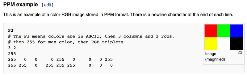
Figure 1: PPM Example

Let’s make some C++ code to output such a thing:

#include <iostream>
 
int main() {
 
    // Image
 
    int image_width = 256;
    int image_height = 256;
 
    // Render
 
    std::cout << "P3\n" << image_width << ' ' << image_height << "\n255\n";
 
    for (int j = 0; j < image_height; j++) {
        for (int i = 0; i < image_width; i++) {
            auto r = double(i) / (image_width-1);
            auto g = double(j) / (image_height-1);
            auto b = 0.0;
 
            int ir = int(255.999 * r);
            int ig = int(255.999 * g);
            int ib = int(255.999 * b);
 
            std::cout << ir << ' ' << ig << ' ' << ib << '\n';
        }
    }
}

Listing 1: [main.cc] Creating your first image

There are some things to note in this code:

1. The pixels are written out in rows.
2. Every row of pixels is written out left to right.
3. These rows are written out from top to bottom.
4. By convention, each of the red/green/blue components are represented internally by real-valued variables that range from 0.0 to 1.0. These must be scaled to integer values between 0 and 255 before we print them out.
5. Red goes from fully off (black) to fully on (bright red) from left to right, and green goes from fully off at the top (black) to fully on at the bottom (bright green). Adding red and green light together make yellow so we should expect the bottom right corner to be yellow.

   

Creating an Image File

Because the file is written to the standard output stream, you’ll need to redirect it to an image file. Typically this is done from the command-line by using the > redirection operator.

On Windows, you’d get the debug build from CMake running this command:

cmake -B build
cmake --build build

Then run your newly-built program like so:

build\Debug\inOneWeekend.exe > image.ppm

Later, it will be better to run optimized builds for speed. In that case, you would build like this:

cmake --build build --config release

and would run the optimized program like this:

build\Release\inOneWeekend.exe > image.ppm

The examples above assume that you are building with CMake, using the same approach as the CMakeLists.txt file in the included source. Use whatever build environment (and language) you’re most comfortable with.

On Mac or Linux, release build, you would launch the program like this:

build/inOneWeekend > image.ppm

Complete building and running instructions can be found in the project README.

Opening the output file (in ToyViewer on my Mac, but try it in your favorite image viewer and Google “ppm viewer” if your viewer doesn’t support it) shows this result:

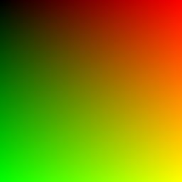
Image 1: First PPM image

Hooray! This is the graphics “hello world”. If your image doesn’t look like that, open the output file in a text editor and see what it looks like. It should start something like this:

 

P3
256 256
255
0 0 0
1 0 0
2 0 0
3 0 0
4 0 0
5 0 0
6 0 0
7 0 0
8 0 0
9 0 0
10 0 0
11 0 0
12 0 0
...

Listing 2: First image output

If your PPM file doesn’t look like this, then double-check your formatting code. If it does look like this but fails to render, then you may have line-ending differences or something similar that is confusing your image viewer. To help debug this, you can find a file test.ppm in the images directory of the Github project. This should help to ensure that your viewer can handle the PPM format and to use as a comparison against your generated PPM file.

Some readers have reported problems viewing their generated files on Windows. In this case, the problem is often that the PPM is written out as UTF-16, often from PowerShell. If you run into this problem, see Discussion 1114 for help with this issue.

If everything displays correctly, then you’re pretty much done with system and IDE issues — everything in the remainder of this series uses this same simple mechanism for generated rendered images.

If you want to produce other image formats, I am a fan of stb_image.h, a header-only image library available on GitHub at https://github.com/nothings/stb.

   

Adding a Progress Indicator

Before we continue, let’s add a progress indicator to our output. This is a handy way to track the progress of a long render, and also to possibly identify a run that’s stalled out due to an infinite loop or other problem.

Our program outputs the image to the standard output stream (std::cout), so leave that alone and instead write to the logging output stream (std::clog):

    for (int j = 0; j < image_height; ++j) {        std::clog << "\rScanlines remaining: " << (image_height - j) << ' ' << std::flush;        for (int i = 0; i < image_width; i++) {
            auto r = double(i) / (image_width-1);
            auto g = double(j) / (image_height-1);
            auto b = 0.0;
 
            int ir = int(255.999 * r);
            int ig = int(255.999 * g);
            int ib = int(255.999 * b);
 
            std::cout << ir << ' ' << ig << ' ' << ib << '\n';
        }
    }
 
    std::clog << "\rDone.                 \n";

Listing 3: [main.cc] Main render loop with progress reporting

Now when running, you’ll see a running count of the number of scanlines remaining. Hopefully this runs so fast that you don’t even see it! Don’t worry — you’ll have lots of time in the future to watch a slowly updating progress line as we expand our ray tracer.

   

The vec3 Class

Almost all graphics programs have some class(es) for storing geometric vectors and colors. In many systems these vectors are 4D (3D position plus a homogeneous coordinate for geometry, or RGB plus an alpha transparency component for colors). For our purposes, three coordinates suffice. We’ll use the same class vec3 for colors, locations, directions, offsets, whatever. Some people don’t like this because it doesn’t prevent you from doing something silly, like subtracting a position from a color. They have a good point, but we’re going to always take the “less code” route when not obviously wrong. In spite of this, we do declare two aliases for vec3: point3 and color. Since these two types are just aliases for vec3, you won’t get warnings if you pass a color to a function expecting a point3, and nothing is stopping you from adding a point3 to a color, but it makes the code a little bit easier to read and to understand.

We define the vec3 class in the top half of a new vec3.h header file, and define a set of useful vector utility functions in the bottom half:

 

#ifndef VEC3_H
#define VEC3_H
 
#include <cmath>
#include <iostream>
 
class vec3 {
  public:
    double e[3];
 
    vec3() : e{0,0,0} {}
    vec3(double e0, double e1, double e2) : e{e0, e1, e2} {}
 
    double x() const { return e[0]; }
    double y() const { return e[1]; }
    double z() const { return e[2]; }
 
    vec3 operator-() const { return vec3(-e[0], -e[1], -e[2]); }
    double operator const { return e[i]; }
    double& operator { return e[i]; }
 
    vec3& operator+=(const vec3& v) {
        e[0] += v.e[0];
        e[1] += v.e[1];
        e[2] += v.e[2];
        return *this;
    }
 
    vec3& operator*=(double t) {
        e[0] *= t;
        e[1] *= t;
        e[2] *= t;
        return *this;
    }
 
    vec3& operator/=(double t) {
        return *this *= 1/t;
    }
 
    double length() const {
        return std::sqrt(length_squared());
    }
 
    double length_squared() const {
        return e[0]*e[0] + e[1]*e[1] + e[2]*e[2];
    }
};
 
// point3 is just an alias for vec3, but useful for geometric clarity in the code.
using point3 = vec3;
 
// Vector Utility Functions
 
inline std::ostream& operator<<(std::ostream& out, const vec3& v) {
    return out << v.e[0] << ' ' << v.e[1] << ' ' << v.e[2];
}
 
inline vec3 operator+(const vec3& u, const vec3& v) {
    return vec3(u.e[0] + v.e[0], u.e[1] + v.e[1], u.e[2] + v.e[2]);
}
 
inline vec3 operator-(const vec3& u, const vec3& v) {
    return vec3(u.e[0] - v.e[0], u.e[1] - v.e[1], u.e[2] - v.e[2]);
}
 
inline vec3 operator*(const vec3& u, const vec3& v) {
    return vec3(u.e[0] * v.e[0], u.e[1] * v.e[1], u.e[2] * v.e[2]);
}
 
inline vec3 operator*(double t, const vec3& v) {
    return vec3(t*v.e[0], t*v.e[1], t*v.e[2]);
}
 
inline vec3 operator*(const vec3& v, double t) {
    return t * v;
}
 
inline vec3 operator/(const vec3& v, double t) {
    return (1/t) * v;
}
 
inline double dot(const vec3& u, const vec3& v) {
    return u.e[0] * v.e[0]
         + u.e[1] * v.e[1]
         + u.e[2] * v.e[2];
}
 
inline vec3 cross(const vec3& u, const vec3& v) {
    return vec3(u.e[1] * v.e[2] - u.e[2] * v.e[1],
                u.e[2] * v.e[0] - u.e[0] * v.e[2],
                u.e[0] * v.e[1] - u.e[1] * v.e[0]);
}
 
inline vec3 unit_vector(const vec3& v) {
    return v / v.length();
}
 
#endif

Listing 4: [vec3.h] vec3 definitions and helper functions

We use double here, but some ray tracers use float. double has greater precision and range, but is twice the size compared to float. This increase in size may be important if you’re programming in limited memory conditions (such as hardware shaders). Either one is fine — follow your own tastes.

   

Color Utility Functions

Using our new vec3 class, we’ll create a new color.h header file and define a utility function that writes a single pixel’s color out to the standard output stream.

 

#ifndef COLOR_H
#define COLOR_H
 
#include "vec3.h"
 
#include <iostream>
 
using color = vec3;
 
void write_color(std::ostream& out, const color& pixel_color) {
    auto r = pixel_color.x();
    auto g = pixel_color.y();
    auto b = pixel_color.z();
 
    // Translate the [0,1] component values to the byte range [0,255].
    int rbyte = int(255.999 * r);
    int gbyte = int(255.999 * g);
    int bbyte = int(255.999 * b);
 
    // Write out the pixel color components.
    out << rbyte << ' ' << gbyte << ' ' << bbyte << '\n';
}
 
#endif

Listing 5: [color.h] color utility functions

Now we can change our main to use both of these:

#include "color.h"
#include "vec3.h"
#include <iostream>
 
int main() {
 
    // Image
 
    int image_width = 256;
    int image_height = 256;
 
    // Render
 
    std::cout << "P3\n" << image_width << ' ' << image_height << "\n255\n";
 
    for (int j = 0; j < image_height; j++) {
        std::clog << "\rScanlines remaining: " << (image_height - j) << ' ' << std::flush;
        for (int i = 0; i < image_width; i++) {            auto pixel_color = color(double(i)/(image_width-1), double(j)/(image_height-1), 0);
            write_color(std::cout, pixel_color);        }
    }
 
    std::clog << "\rDone.                 \n";
}

Listing 6: [main.cc] Final code for the first PPM image

And you should get the exact same picture as before.

   

Rays, a Simple Camera, and Background

   

The ray Class

The one thing that all ray tracers have is a ray class and a computation of what color is seen along a ray. Let’s think of a ray as a function $\mathbf{P}(t)=\mathbf{A}+t\mathbf{b}$. Here $\mathbf{P}$ is a 3D position along a line in 3D. $\mathbf{A}$ is the ray origin and $\mathbf{b}$ is the ray direction. The ray parameter $t$ is a real number (double in the code). Plug in a different $t$ and $\mathbf{P}(t)$ moves the point along the ray. Add in negative $t$ values and you can go anywhere on the 3D line. For positive $t$, you get only the parts in front of $\mathbf{A}$, and this is what is often called a half-line or a ray.

 

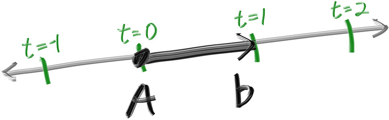
Figure 2: Linear interpolation

We can represent the idea of a ray as a class, and represent the function $\mathbf{P}(t)$ as a function that we’ll call ray::at(t):

#ifndef RAY_H
#define RAY_H
 
#include "vec3.h"
 
class ray {
  public:
    ray() {}
 
    ray(const point3& origin, const vec3& direction) : orig(origin), dir(direction) {}
 
    const point3& origin() const  { return orig; }
    const vec3& direction() const { return dir; }
 
    point3 at(double t) const {
        return orig + t*dir;
    }
 
  private:
    point3 orig;
    vec3 dir;
};
 
#endif

Listing 7: [ray.h] The ray class

(For those unfamiliar with C++, the functions ray::origin() and ray::direction() both return an immutable reference to their members. Callers can either just use the reference directly, or make a mutable copy depending on their needs.)

   

Sending Rays Into the Scene

Now we are ready to turn the corner and make a ray tracer. At its core, a ray tracer sends rays through pixels and computes the color seen in the direction of those rays. The involved steps are

1. Calculate the ray from the “eye” through the pixel,
2. Determine which objects the ray intersects, and
3. Compute a color for the closest intersection point.

When first developing a ray tracer, I always do a simple camera for getting the code up and running.

I’ve often gotten into trouble using square images for debugging because I transpose $x$ and $y$ too often, so we’ll use a non-square image. A square image has a 1∶1 aspect ratio, because its width is the same as its height. Since we want a non-square image, we’ll choose 16∶9 because it’s so common. A 16∶9 aspect ratio means that the ratio of image width to image height is 16∶9. Put another way, given an image with a 16∶9 aspect ratio,

$$\text{width}/\text{height}=16/9=1.7778$$

For a practical example, an image 800 pixels wide by 400 pixels high has a 2∶1 aspect ratio.

The image’s aspect ratio can be determined from the ratio of its width to its height. However, since we have a given aspect ratio in mind, it’s easier to set the image’s width and the aspect ratio, and then using this to calculate for its height. This way, we can scale up or down the image by changing the image width, and it won’t throw off our desired aspect ratio. We do have to make sure that when we solve for the image height the resulting height is at least 1.

In addition to setting up the pixel dimensions for the rendered image, we also need to set up a virtual viewport through which to pass our scene rays. The viewport is a virtual rectangle in the 3D world that contains the grid of image pixel locations. If pixels are spaced the same distance horizontally as they are vertically, the viewport that bounds them will have the same aspect ratio as the rendered image. The distance between two adjacent pixels is called the pixel spacing, and square pixels is the standard.

To start things off, we’ll choose an arbitrary viewport height of 2.0, and scale the viewport width to give us the desired aspect ratio. Here’s a snippet of what this code will look like:

 

auto aspect_ratio = 16.0 / 9.0;
int image_width = 400;
 
// Calculate the image height, and ensure that it's at least 1.
int image_height = int(image_width / aspect_ratio);
image_height = (image_height < 1) ? 1 : image_height;
 
// Viewport widths less than one are ok since they are real valued.
auto viewport_height = 2.0;
auto viewport_width = viewport_height * (double(image_width)/image_height);

Listing 8: Rendered image setup

If you’re wondering why we don’t just use aspect_ratio when computing viewport_width, it’s because the value set to aspect_ratio is the ideal ratio, it may not be the actual ratio between image_width and image_height. If image_height was allowed to be real valued—rather than just an integer—then it would be fine to use aspect_ratio. But the actual ratio between image_width and image_height can vary based on two parts of the code. First, image_height is rounded down to the nearest integer, which can increase the ratio. Second, we don’t allow image_height to be less than one, which can also change the actual aspect ratio.

Note that aspect_ratio is an ideal ratio, which we approximate as best as possible with the integer-based ratio of image width over image height. In order for our viewport proportions to exactly match our image proportions, we use the calculated image aspect ratio to determine our final viewport width.

Next we will define the camera center: a point in 3D space from which all scene rays will originate (this is also commonly referred to as the eye point). The vector from the camera center to the viewport center will be orthogonal to the viewport. We’ll initially set the distance between the viewport and the camera center point to be one unit. This distance is often referred to as the focal length.

For simplicity we’ll start with the camera center at $(0,0,0)$. We’ll also have the y-axis go up, the x-axis to the right, and the negative z-axis pointing in the viewing direction. (This is commonly referred to as right-handed coordinates.)

 

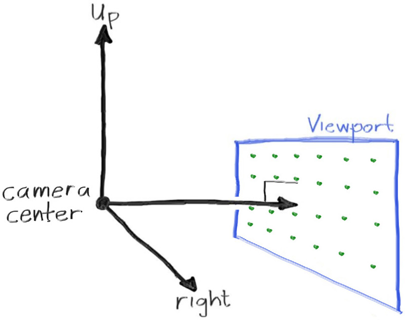
Figure 3: Camera geometry

Now the inevitable tricky part. While our 3D space has the conventions above, this conflicts with our image coordinates, where we want to have the zeroth pixel in the top-left and work our way down to the last pixel at the bottom right. This means that our image coordinate Y-axis is inverted: Y increases going down the image.

As we scan our image, we will start at the upper left pixel (pixel $0,0$), scan left-to-right across each row, and then scan row-by-row, top-to-bottom. To help navigate the pixel grid, we’ll use a vector from the left edge to the right edge (${\left(\mathbf{V}\right)}_{\mathbf{u}}$), and a vector from the upper edge to the lower edge (${\left(\mathbf{V}\right)}_{\mathbf{v}}$).

Our pixel grid will be inset from the viewport edges by half the pixel-to-pixel distance. This way, our viewport area is evenly divided into width × height identical regions. Here’s what our viewport and pixel grid look like:

 

Figure 4: Viewport and pixel grid

In this figure, we have the viewport, the pixel grid for a 7×5 resolution image, the viewport upper left corner $\mathbf{Q}$, the pixel ${\left(\mathbf{P}\right)}_{0,0}$ location, the viewport vector ${\left(\mathbf{V}\right)}_{\mathbf{u}}$ (viewport_u), the viewport vector ${\left(\mathbf{V}\right)}_{\mathbf{v}}$ (viewport_v), and the pixel delta vectors $\mathbf{\Delta u}$ and $\mathbf{\Delta v}$.

Drawing from all of this, here’s the code that implements the camera. We’ll stub in a function ray_color(const ray& r) that returns the color for a given scene ray — which we’ll set to always return black for now.

#include "color.h"#include "ray.h"#include "vec3.h"
 
#include <iostream>
 
color ray_color(const ray& r) {
    return color(0,0,0);
}
int main() {
 
    // Image
 
    auto aspect_ratio = 16.0 / 9.0;
    int image_width = 400;
 
    // Calculate the image height, and ensure that it's at least 1.
    int image_height = int(image_width / aspect_ratio);
    image_height = (image_height < 1) ? 1 : image_height;
 
    // Camera
 
    auto focal_length = 1.0;
    auto viewport_height = 2.0;
    auto viewport_width = viewport_height * (double(image_width)/image_height);
    auto camera_center = point3(0, 0, 0);
 
    // Calculate the vectors across the horizontal and down the vertical viewport edges.
    auto viewport_u = vec3(viewport_width, 0, 0);
    auto viewport_v = vec3(0, -viewport_height, 0);
 
    // Calculate the horizontal and vertical delta vectors from pixel to pixel.
    auto pixel_delta_u = viewport_u / image_width;
    auto pixel_delta_v = viewport_v / image_height;
 
    // Calculate the location of the upper left pixel.
    auto viewport_upper_left = camera_center
                             - vec3(0, 0, focal_length) - viewport_u/2 - viewport_v/2;
    auto pixel00_loc = viewport_upper_left + 0.5 * (pixel_delta_u + pixel_delta_v);
    // Render
 
    std::cout << "P3\n" << image_width << " " << image_height << "\n255\n";
 
    for (int j = 0; j < image_height; j++) {
        std::clog << "\rScanlines remaining: " << (image_height - j) << ' ' << std::flush;
        for (int i = 0; i < image_width; i++) {            auto pixel_center = pixel00_loc + (i * pixel_delta_u) + (j * pixel_delta_v);
            auto ray_direction = pixel_center - camera_center;
            ray r(camera_center, ray_direction);
 
            color pixel_color = ray_color(r);            write_color(std::cout, pixel_color);
        }
    }
 
    std::clog << "\rDone.                 \n";
}

Listing 9: [main.cc] Creating scene rays

Notice that in the code above, I didn’t make ray_direction a unit vector, because I think not doing that makes for simpler and slightly faster code.

Now we’ll fill in the ray_color(ray) function to implement a simple gradient. This function will linearly blend white and blue depending on the height of the $y$ coordinate after scaling the ray direction to unit length (so $-1.0<y<1.0$). Because we’re looking at the $y$ height after normalizing the vector, you’ll notice a horizontal gradient to the color in addition to the vertical gradient.

I’ll use a standard graphics trick to linearly scale $0.0\le a\le 1.0$. When $a=1.0$, I want blue. When $a=0.0$, I want white. In between, I want a blend. This forms a “linear blend”, or “linear interpolation”. This is commonly referred to as a lerp between two values. A lerp is always of the form

$$blendedValue=(1-a)\cdot startValue+a\cdot endValue,$$

with $a$ going from zero to one.

Putting all this together, here’s what we get:

#include "color.h"
#include "ray.h"
#include "vec3.h"
 
#include <iostream>
 
color ray_color(const ray& r) {    vec3 unit_direction = unit_vector(r.direction());
    auto a = 0.5*(unit_direction.y() + 1.0);
    return (1.0-a)*color(1.0, 1.0, 1.0) + a*color(0.5, 0.7, 1.0);}
 
...

Listing 10: [main.cc] Rendering a blue-to-white gradient

In our case this produces:

Image 2: A blue-to-white gradient depending on ray Y coordinate

   

Adding a Sphere

Let’s add a single object to our ray tracer. People often use spheres in ray tracers because calculating whether a ray hits a sphere is relatively simple.

   

Ray-Sphere Intersection

The equation for a sphere of radius $r$ that is centered at the origin is an important mathematical equation:

$$x^2+y^2+z^2=r^2$$

You can also think of this as saying that if a given point $(x,y,z)$ is on the surface of the sphere, then $x^2+y^2+z^2=r^2$. If a given point $(x,y,z)$ is inside the sphere, then $x^2+y^2+z^2<r^2$, and if a given point $(x,y,z)$ is outside the sphere, then $x^2+y^2+z^2>r^2$.

If we want to allow the sphere center to be at an arbitrary point $(C_x,C_y,C_z)$, then the equation becomes a lot less nice:

$$(C_x-x{\left()\right)}^2+(C_y-y{\left()\right)}^2+(C_z-z{\left()\right)}^2=r^2$$

In graphics, you almost always want your formulas to be in terms of vectors so that all the $x$/$y$/$z$ stuff can be simply represented using a vec3 class. You might note that the vector from point $\mathbf{P}=(x,y,z)$ to center $\mathbf{C}=(C_x,C_y,C_z)$ is $(\mathbf{C}-\mathbf{P})$.

If we use the definition of the dot product:

$$(\mathbf{C}-\mathbf{P})\cdot (\mathbf{C}-\mathbf{P})=(C_x-x{\left()\right)}^2+(C_y-y{\left()\right)}^2+(C_z-z{\left()\right)}^2$$

Then we can rewrite the equation of the sphere in vector form as:

$$(\mathbf{C}-\mathbf{P})\cdot (\mathbf{C}-\mathbf{P})=r^2$$

We can read this as “any point $\mathbf{P}$ that satisfies this equation is on the sphere”. We want to know if our ray $\mathbf{P}(t)=\mathbf{Q}+t\mathbf{d}$ ever hits the sphere anywhere. If it does hit the sphere, there is some $t$ for which $\mathbf{P}(t)$ satisfies the sphere equation. So we are looking for any $t$ where this is true:

$$(\mathbf{C}-\mathbf{P}(t))\cdot (\mathbf{C}-\mathbf{P}(t))=r^2$$

which can be found by replacing $\mathbf{P}(t)$ with its expanded form:

$$(\mathbf{C}-(\mathbf{Q}+t\mathbf{d}))\cdot (\mathbf{C}-(\mathbf{Q}+t\mathbf{d}))=r^2$$

We have three vectors on the left dotted by three vectors on the right. If we solved for the full dot product we would get nine vectors. You can definitely go through and write everything out, but we don’t need to work that hard. If you remember, we want to solve for $t$, so we’ll separate the terms based on whether there is a $t$ or not:

$$(-t\mathbf{d}+(\mathbf{C}-\mathbf{Q}))\cdot (-t\mathbf{d}+(\mathbf{C}-\mathbf{Q}))=r^2$$

And now we follow the rules of vector algebra to distribute the dot product:

$$t^2\mathbf{d}\cdot \mathbf{d}-2t\mathbf{d}\cdot (\mathbf{C}-\mathbf{Q})+(\mathbf{C}-\mathbf{Q})\cdot (\mathbf{C}-\mathbf{Q})=r^2$$

Move the square of the radius over to the left hand side:

$$t^2\mathbf{d}\cdot \mathbf{d}-2t\mathbf{d}\cdot (\mathbf{C}-\mathbf{Q})+(\mathbf{C}-\mathbf{Q})\cdot (\mathbf{C}-\mathbf{Q})-r^2=0$$

It’s hard to make out what exactly this equation is, but the vectors and $r$ in that equation are all constant and known. Furthermore, the only vectors that we have are reduced to scalars by dot product. The only unknown is $t$, and we have a $t^2$, which means that this equation is quadratic. You can solve for a quadratic equation $a{x}^2+bx+c=0$ by using the quadratic formula:

$$\frac{-b\pm \sqrt{b^2-4ac}}{2a}$$

So solving for $t$ in the ray-sphere intersection equation gives us these values for $a$, $b$, and $c$:

$$a=\mathbf{d}\cdot \mathbf{d}$$ $$b=-2\mathbf{d}\cdot (\mathbf{C}-\mathbf{Q})$$ $$c=(\mathbf{C}-\mathbf{Q})\cdot (\mathbf{C}-\mathbf{Q})-r^2$$

Using all of the above you can solve for $t$, but there is a square root part that can be either positive (meaning two real solutions), negative (meaning no real solutions), or zero (meaning one real solution). In graphics, the algebra almost always relates very directly to the geometry. What we have is:

 

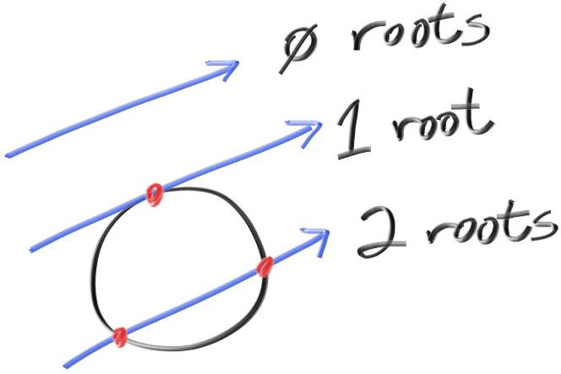
Figure 5: Ray-sphere intersection results

   

Creating Our First Raytraced Image

If we take that math and hard-code it into our program, we can test our code by placing a small sphere at −1 on the z-axis and then coloring red any pixel that intersects it.

 

bool hit_sphere(const point3& center, double radius, const ray& r) {
    vec3 oc = center - r.origin();
    auto a = dot(r.direction(), r.direction());
    auto b = -2.0 * dot(r.direction(), oc);
    auto c = dot(oc, oc) - radius*radius;
    auto discriminant = b*b - 4*a*c;
    return (discriminant >= 0);
}
color ray_color(const ray& r) {    if (hit_sphere(point3(0,0,-1), 0.5, r))
        return color(1, 0, 0);
    vec3 unit_direction = unit_vector(r.direction());
    auto a = 0.5*(unit_direction.y() + 1.0);
    return (1.0-a)*color(1.0, 1.0, 1.0) + a*color(0.5, 0.7, 1.0);
}

Listing 11: [main.cc] Rendering a red sphere

What we get is this:

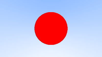
Image 3: A simple red sphere

Now this lacks all sorts of things — like shading, reflection rays, and more than one object — but we are closer to halfway done than we are to our start! One thing to be aware of is that we are testing to see if a ray intersects with the sphere by solving the quadratic equation and seeing if a solution exists, but solutions with negative values of $t$ work just fine. If you change your sphere center to $z=+1$ you will get exactly the same picture because this solution doesn’t distinguish between objects in front of the camera and objects behind the camera. This is not a feature! We’ll fix those issues next.

   

Surface Normals and Multiple Objects

   

Shading with Surface Normals

First, let’s get ourselves a surface normal so we can shade. This is a vector that is perpendicular to the surface at the point of intersection.

We have a key design decision to make for normal vectors in our code: whether normal vectors will have an arbitrary length, or will be normalized to unit length.

It is tempting to skip the expensive square root operation involved in normalizing the vector, in case it’s not needed. In practice, however, there are three important observations. First, if a unit-length normal vector is ever required, then you might as well do it up front once, instead of over and over again “just in case” for every location where unit-length is required. Second, we do require unit-length normal vectors in several places. Third, if you require normal vectors to be unit length, then you can often efficiently generate that vector with an understanding of the specific geometry class, in its constructor, or in the hit() function. For example, sphere normals can be made unit length simply by dividing by the sphere radius, avoiding the square root entirely.

Given all of this, we will adopt the policy that all normal vectors will be of unit length.

For a sphere, the outward normal is in the direction of the hit point minus the center:

 

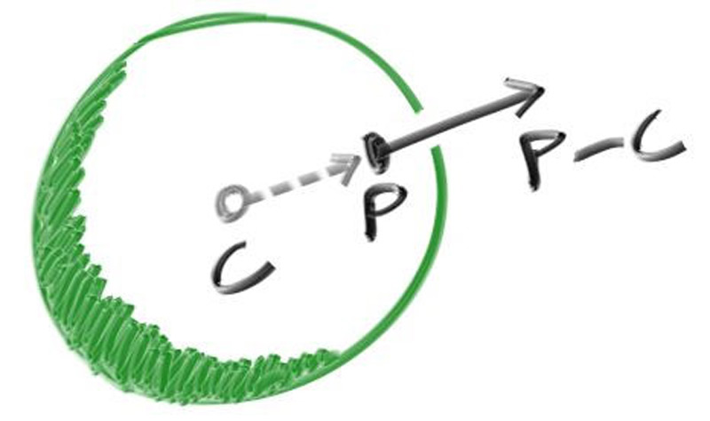
Figure 6: Sphere surface-normal geometry

On the earth, this means that the vector from the earth’s center to you points straight up. Let’s throw that into the code now, and shade it. We don’t have any lights or anything yet, so let’s just visualize the normals with a color map. A common trick used for visualizing normals (because it’s easy and somewhat intuitive to assume $\mathbf{n}$ is a unit length vector — so each component is between −1 and 1) is to map each component to the interval from 0 to 1, and then map $(x,y,z)$ to $(red,green,blue)$. For the normal, we need the hit point, not just whether we hit or not (which is all we’re calculating at the moment). We only have one sphere in the scene, and it’s directly in front of the camera, so we won’t worry about negative values of $t$ yet. We’ll just assume the closest hit point (smallest $t$) is the one that we want. These changes in the code let us compute and visualize $\mathbf{n}$:

 

double hit_sphere(const point3& center, double radius, const ray& r) {    vec3 oc = center - r.origin();
    auto a = dot(r.direction(), r.direction());
    auto b = -2.0 * dot(r.direction(), oc);
    auto c = dot(oc, oc) - radius*radius;
    auto discriminant = b*b - 4*a*c;
 
    if (discriminant < 0) {
        return -1.0;
    } else {
        return (-b - std::sqrt(discriminant) ) / (2.0*a);
    }}
 
color ray_color(const ray& r) {    auto t = hit_sphere(point3(0,0,-1), 0.5, r);
    if (t > 0.0) {
        vec3 N = unit_vector(r.at(t) - vec3(0,0,-1));
        return 0.5*color(N.x()+1, N.y()+1, N.z()+1);
    }
    vec3 unit_direction = unit_vector(r.direction());
    auto a = 0.5*(unit_direction.y() + 1.0);
    return (1.0-a)*color(1.0, 1.0, 1.0) + a*color(0.5, 0.7, 1.0);
}

Listing 12: [main.cc] Rendering surface normals on a sphere

And that yields this picture:

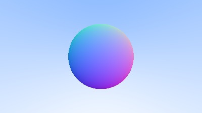
Image 4: A sphere colored according to its normal vectors

   

Simplifying the Ray-Sphere Intersection Code

Let’s revisit the ray-sphere function:

 

double hit_sphere(const point3& center, double radius, const ray& r) {
    vec3 oc = center - r.origin();
    auto a = dot(r.direction(), r.direction());
    auto b = -2.0 * dot(r.direction(), oc);
    auto c = dot(oc, oc) - radius*radius;
    auto discriminant = b*b - 4*a*c;
 
    if (discriminant < 0) {
        return -1.0;
    } else {
        return (-b - std::sqrt(discriminant) ) / (2.0*a);
    }
}

Listing 13: [main.cc] Ray-sphere intersection code (before)

First, recall that a vector dotted with itself is equal to the squared length of that vector.

Second, notice how the equation for b has a factor of negative two in it. Consider what happens to the quadratic equation if $b=-2h$:

$$\frac{-b\pm \sqrt{b^2-4ac}}{2a}$$ $$=\frac{-(-2h)\pm \sqrt{(-2h{\left()\right)}^2-4ac}}{2a}$$ $$=\frac{2h\pm 2\sqrt{h^2-ac}}{2a}$$ $$=\frac{h\pm \sqrt{h^2-ac}}{a}$$

This simplifies nicely, so we’ll use it. So solving for $h$:

$$b=-2\mathbf{d}\cdot (\mathbf{C}-\mathbf{Q})$$ $$b=-2h$$ $$h=\frac{b}{-2}=\mathbf{d}\cdot (\mathbf{C}-\mathbf{Q})$$

Using these observations, we can now simplify the sphere-intersection code to this:

double hit_sphere(const point3& center, double radius, const ray& r) {
    vec3 oc = center - r.origin();    auto a = r.direction().length_squared();
    auto h = dot(r.direction(), oc);
    auto c = oc.length_squared() - radius*radius;
    auto discriminant = h*h - a*c;
    if (discriminant < 0) {
        return -1.0;
    } else {        return (h - std::sqrt(discriminant)) / a;    }
}

Listing 14: [main.cc] Ray-sphere intersection code (after)

   

An Abstraction for Hittable Objects

Now, how about more than one sphere? While it is tempting to have an array of spheres, a very clean solution is to make an “abstract class” for anything a ray might hit, and make both a sphere and a list of spheres just something that can be hit. What that class should be called is something of a quandary — calling it an “object” would be good if not for “object oriented” programming. “Surface” is often used, with the weakness being maybe we will want volumes (fog, clouds, stuff like that). “hittable” emphasizes the member function that unites them. I don’t love any of these, but we’ll go with “hittable”.

This hittable abstract class will have a hit function that takes in a ray. Most ray tracers have found it convenient to add a valid interval for hits $t_{min}$ to $t_{max}$, so the hit only “counts” if $t_{min}<t<t_{max}$. For the initial rays this is positive $t$, but as we will see, it can simplify our code to have an interval $t_{min}$ to $t_{max}$. One design question is whether to do things like compute the normal if we hit something. We might end up hitting something closer as we do our search, and we will only need the normal of the closest thing. I will go with the simple solution and compute a bundle of stuff I will store in some structure. Here’s the abstract class:

 

#ifndef HITTABLE_H
#define HITTABLE_H
 
#include "ray.h"
 
class hit_record {
  public:
    point3 p;
    vec3 normal;
    double t;
};
 
class hittable {
  public:
    virtual ~hittable() = default;
 
    virtual bool hit(const ray& r, double ray_tmin, double ray_tmax, hit_record& rec) const = 0;
};
 
#endif

Listing 15: [hittable.h] The hittable class

And here’s the sphere:

#ifndef SPHERE_H
#define SPHERE_H
 
#include "hittable.h"
#include "vec3.h"
 
class sphere : public hittable {
  public:
    sphere(const point3& center, double radius) : center(center), radius(std::fmax(0,radius)) {}
 
    bool hit(const ray& r, double ray_tmin, double ray_tmax, hit_record& rec) const override {
        vec3 oc = center - r.origin();
        auto a = r.direction().length_squared();
        auto h = dot(r.direction(), oc);
        auto c = oc.length_squared() - radius*radius;
 
        auto discriminant = h*h - a*c;
        if (discriminant < 0)
            return false;
 
        auto sqrtd = std::sqrt(discriminant);
 
        // Find the nearest root that lies in the acceptable range.
        auto root = (h - sqrtd) / a;
        if (root <= ray_tmin || ray_tmax <= root) {
            root = (h + sqrtd) / a;
            if (root <= ray_tmin || ray_tmax <= root)
                return false;
        }
 
        rec.t = root;
        rec.p = r.at(rec.t);
        rec.normal = (rec.p - center) / radius;
 
        return true;
    }
 
  private:
    point3 center;
    double radius;
};
 
#endif

Listing 16: [sphere.h] The sphere class

(Note here that we use the C++ standard function std::fmax(), which returns the maximum of the two floating-point arguments. Similarly, we will later use std::fmin(), which returns the minimum of the two floating-point arguments.)

   

Front Faces Versus Back Faces

The second design decision for normals is whether they should always point out. At present, the normal found will always be in the direction of the center to the intersection point (the normal points out). If the ray intersects the sphere from the outside, the normal points against the ray. If the ray intersects the sphere from the inside, the normal (which always points out) points with the ray. Alternatively, we can have the normal always point against the ray. If the ray is outside the sphere, the normal will point outward, but if the ray is inside the sphere, the normal will point inward.

 

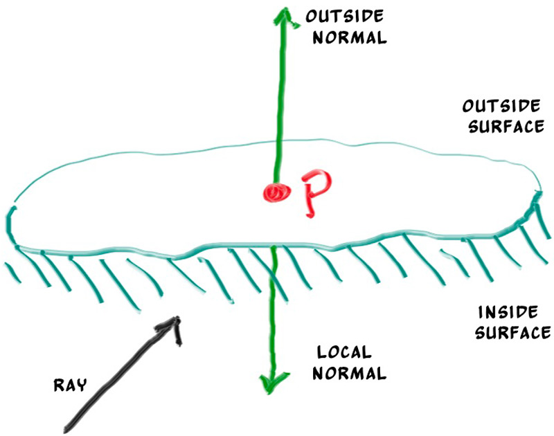
Figure 7: Possible directions for sphere surface-normal geometry

We need to choose one of these possibilities because we will eventually want to determine which side of the surface that the ray is coming from. This is important for objects that are rendered differently on each side, like the text on a two-sided sheet of paper, or for objects that have an inside and an outside, like glass balls.

If we decide to have the normals always point out, then we will need to determine which side the ray is on when we color it. We can figure this out by comparing the ray with the normal. If the ray and the normal face in the same direction, the ray is inside the object, if the ray and the normal face in the opposite direction, then the ray is outside the object. This can be determined by taking the dot product of the two vectors, where if their dot is positive, the ray is inside the sphere.

 

if (dot(ray_direction, outward_normal) > 0.0) {
    // ray is inside the sphere
    ...
} else {
    // ray is outside the sphere
    ...
}

Listing 17: Comparing the ray and the normal

If we decide to have the normals always point against the ray, we won’t be able to use the dot product to determine which side of the surface the ray is on. Instead, we would need to store that information:

bool front_face;
if (dot(ray_direction, outward_normal) > 0.0) {
    // ray is inside the sphere
    normal = -outward_normal;
    front_face = false;
} else {
    // ray is outside the sphere
    normal = outward_normal;
    front_face = true;
}

Listing 18: Remembering the side of the surface

We can set things up so that normals always point “outward” from the surface, or always point against the incident ray. This decision is determined by whether you want to determine the side of the surface at the time of geometry intersection or at the time of coloring. In this book we have more material types than we have geometry types, so we’ll go for less work and put the determination at geometry time. This is simply a matter of preference, and you’ll see both implementations in the literature.

We add the front_face bool to the hit_record class. We’ll also add a function to solve this calculation for us: set_face_normal(). For convenience we will assume that the vector passed to the new set_face_normal() function is of unit length. We could always normalize the parameter explicitly, but it’s more efficient if the geometry code does this, as it’s usually easier when you know more about the specific geometry.

 

class hit_record {
  public:
    point3 p;
    vec3 normal;
    double t;    bool front_face;
 
    void set_face_normal(const ray& r, const vec3& outward_normal) {
        // Sets the hit record normal vector.
        // NOTE: the parameter \`outward_normal\` is assumed to have unit length.
 
        front_face = dot(r.direction(), outward_normal) < 0;
        normal = front_face ? outward_normal : -outward_normal;
    }};

Listing 19: [hittable.h] Adding front-face tracking to hit_record

And then we add the surface side determination to the class:

class sphere : public hittable {
  public:
    ...
    bool hit(const ray& r, double ray_tmin, double ray_tmax, hit_record& rec) const {
        ...
 
        rec.t = root;
        rec.p = r.at(rec.t);        vec3 outward_normal = (rec.p - center) / radius;
        rec.set_face_normal(r, outward_normal);
        return true;
    }
    ...
};

Listing 20: [sphere.h] The sphere class with normal determination

   

A List of Hittable Objects

We have a generic object called a hittable that the ray can intersect with. We now add a class that stores a list of hittables:

 

#ifndef HITTABLE_LIST_H
#define HITTABLE_LIST_H
 
#include "hittable.h"
 
#include <memory>
#include <vector>
 
using std::make_shared;
using std::shared_ptr;
 
class hittable_list : public hittable {
  public:
    std::vector<shared_ptr<hittable>> objects;
 
    hittable_list() {}
    hittable_list(shared_ptr<hittable> object) { add(object); }
 
    void clear() { objects.clear(); }
 
    void add(shared_ptr<hittable> object) {
        objects.push_back(object);
    }
 
    bool hit(const ray& r, double ray_tmin, double ray_tmax, hit_record& rec) const override {
        hit_record temp_rec;
        bool hit_anything = false;
        auto closest_so_far = ray_tmax;
 
        for (const auto& object : objects) {
            if (object->hit(r, ray_tmin, closest_so_far, temp_rec)) {
                hit_anything = true;
                closest_so_far = temp_rec.t;
                rec = temp_rec;
            }
        }
 
        return hit_anything;
    }
};
 
#endif

Listing 21: [hittable_list.h] The hittable_list class

   

Some New C++ Features

The hittable_list class code uses some C++ features that may trip you up if you’re not normally a C++ programmer: vector, shared_ptr, and make_shared.

shared_ptr<type> is a pointer to some allocated type, with reference-counting semantics. Every time you assign its value to another shared pointer (usually with a simple assignment), the reference count is incremented. As shared pointers go out of scope (like at the end of a block or function), the reference count is decremented. Once the count goes to zero, the object is safely deleted.

Typically, a shared pointer is first initialized with a newly-allocated object, something like this:

shared_ptr<double> double_ptr = make_shared<double>(0.37);
shared_ptr<vec3>   vec3_ptr   = make_shared<vec3>(1.414214, 2.718281, 1.618034);
shared_ptr<sphere> sphere_ptr = make_shared<sphere>(point3(0,0,0), 1.0);

Listing 22: An example allocation using shared_ptr

make_shared<thing>(thing_constructor_params ...) allocates a new instance of type thing, using the constructor parameters. It returns a shared_ptr<thing>.

Since the type can be automatically deduced by the return type of make_shared<type>(...), the above lines can be more simply expressed using C++‘s auto type specifier:

auto double_ptr = make_shared<double>(0.37);
auto vec3_ptr   = make_shared<vec3>(1.414214, 2.718281, 1.618034);
auto sphere_ptr = make_shared<sphere>(point3(0,0,0), 1.0);

Listing 23: An example allocation using shared_ptr with auto type

We’ll use shared pointers in our code, because it allows multiple geometries to share a common instance (for example, a bunch of spheres that all use the same color material), and because it makes memory management automatic and easier to reason about.

std::shared_ptr is included with the <memory> header.

The second C++ feature you may be unfamiliar with is std::vector. This is a generic array-like collection of an arbitrary type. Above, we use a collection of pointers to hittable. std::vector automatically grows as more values are added: objects.push_back(object) adds a value to the end of the std::vector member variable objects.

std::vector is included with the <vector> header.

Finally, the using statements in listing 21 tell the compiler that we’ll be getting shared_ptr and make_shared from the std library, so we don’t need to prefix these with std:: every time we reference them.

   

Common Constants and Utility Functions

We need some math constants that we conveniently define in their own header file. For now we only need infinity, but we will also throw our own definition of pi in there, which we will need later. We’ll also throw common useful constants and future utility functions in here. This new header, rtweekend.h, will be our general main header file.

 

#ifndef RTWEEKEND_H
#define RTWEEKEND_H
 
#include <cmath>
#include <iostream>
#include <limits>
#include <memory>
 
// C++ Std Usings
 
using std::make_shared;
using std::shared_ptr;
 
// Constants
 
const double infinity = std::numeric_limits<double>::infinity();
const double pi = 3.1415926535897932385;
 
// Utility Functions
 
inline double degrees_to_radians(double degrees) {
    return degrees * pi / 180.0;
}
 
// Common Headers
 
#include "color.h"
#include "ray.h"
#include "vec3.h"
 
#endif

Listing 24: [rtweekend.h] The rtweekend.h common header

Program files will include rtweekend.h first, so all other header files (where the bulk of our code will reside) can implicitly assume that rtweekend.h has already been included. Header files still need to explicitly include any other necessary header files. We’ll make some updates with these assumptions in mind.

 

#include <iostream>

Listing 25: [color.h] Assume rtweekend.h inclusion for color.h

 

#include "ray.h"

Listing 26: [hittable.h] Assume rtweekend.h inclusion for hittable.h

 

#include <memory>#include <vector>
 
using std::make_shared;
using std::shared_ptr;

Listing 27: [hittable_list.h] Assume rtweekend.h inclusion for hittable_list.h

 

#include "vec3.h"

Listing 28: [sphere.h] Assume rtweekend.h inclusion for sphere.h

 

#include <cmath>
#include <iostream>

Listing 29: [vec3.h] Assume rtweekend.h inclusion for vec3.h

And now the new main:

#include "rtweekend.h"
#include "color.h"
#include "ray.h"
#include "vec3.h"#include "hittable.h"
#include "hittable_list.h"
#include "sphere.h"
#include <iostream>
double hit_sphere(const point3& center, double radius, const ray& r) {
    ...
}
color ray_color(const ray& r, const hittable& world) {
    hit_record rec;
    if (world.hit(r, 0, infinity, rec)) {
        return 0.5 * (rec.normal + color(1,1,1));
    }
    vec3 unit_direction = unit_vector(r.direction());
    auto a = 0.5*(unit_direction.y() + 1.0);
    return (1.0-a)*color(1.0, 1.0, 1.0) + a*color(0.5, 0.7, 1.0);
}
 
int main() {
 
    // Image
 
    auto aspect_ratio = 16.0 / 9.0;
    int image_width = 400;
 
    // Calculate the image height, and ensure that it's at least 1.
    int image_height = int(image_width / aspect_ratio);
    image_height = (image_height < 1) ? 1 : image_height;
 
    // World
 
    hittable_list world;
 
    world.add(make_shared<sphere>(point3(0,0,-1), 0.5));
    world.add(make_shared<sphere>(point3(0,-100.5,-1), 100));
    // Camera
 
    auto focal_length = 1.0;
    auto viewport_height = 2.0;
    auto viewport_width = viewport_height * (double(image_width)/image_height);
    auto camera_center = point3(0, 0, 0);
 
    // Calculate the vectors across the horizontal and down the vertical viewport edges.
    auto viewport_u = vec3(viewport_width, 0, 0);
    auto viewport_v = vec3(0, -viewport_height, 0);
 
    // Calculate the horizontal and vertical delta vectors from pixel to pixel.
    auto pixel_delta_u = viewport_u / image_width;
    auto pixel_delta_v = viewport_v / image_height;
 
    // Calculate the location of the upper left pixel.
    auto viewport_upper_left = camera_center
                             - vec3(0, 0, focal_length) - viewport_u/2 - viewport_v/2;
    auto pixel00_loc = viewport_upper_left + 0.5 * (pixel_delta_u + pixel_delta_v);
 
    // Render
 
    std::cout << "P3\n" << image_width << ' ' << image_height << "\n255\n";
 
    for (int j = 0; j < image_height; j++) {
        std::clog << "\rScanlines remaining: " << (image_height - j) << ' ' << std::flush;
        for (int i = 0; i < image_width; i++) {
            auto pixel_center = pixel00_loc + (i * pixel_delta_u) + (j * pixel_delta_v);
            auto ray_direction = pixel_center - camera_center;
            ray r(camera_center, ray_direction);
 
            color pixel_color = ray_color(r, world);            write_color(std::cout, pixel_color);
        }
    }
 
    std::clog << "\rDone.                 \n";
}

Listing 30: [main.cc] The new main with hittables

This yields a picture that is really just a visualization of where the spheres are located along with their surface normal. This is often a great way to view any flaws or specific characteristics of a geometric model.

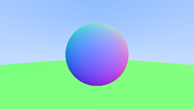
Image 5: Resulting render of normals-colored sphere with ground

   

An Interval Class

Before we continue, we’ll implement an interval class to manage real-valued intervals with a minimum and a maximum. We’ll end up using this class quite often as we proceed.

 

#ifndef INTERVAL_H
#define INTERVAL_H
 
class interval {
  public:
    double min, max;
 
    interval() : min(+infinity), max(-infinity) {} // Default interval is empty
 
    interval(double min, double max) : min(min), max(max) {}
 
    double size() const {
        return max - min;
    }
 
    bool contains(double x) const {
        return min <= x && x <= max;
    }
 
    bool surrounds(double x) const {
        return min < x && x < max;
    }
 
    static const interval empty, universe;
};
 
const interval interval::empty    = interval(+infinity, -infinity);
const interval interval::universe = interval(-infinity, +infinity);
 
#endif

Listing 31: [interval.h] Introducing the new interval class

 

// Common Headers
 
#include "color.h"#include "interval.h"#include "ray.h"
#include "vec3.h"

Listing 32: [rtweekend.h] Including the new interval class

 

class hittable {
  public:
    ...    virtual bool hit(const ray& r, interval ray_t, hit_record& rec) const = 0;};

Listing 33: [hittable.h] hittable::hit() using interval

 

class hittable_list : public hittable {
  public:
    ...    bool hit(const ray& r, interval ray_t, hit_record& rec) const override {        hit_record temp_rec;
        bool hit_anything = false;        auto closest_so_far = ray_t.max;
        for (const auto& object : objects) {            if (object->hit(r, interval(ray_t.min, closest_so_far), temp_rec)) {                hit_anything = true;
                closest_so_far = temp_rec.t;
                rec = temp_rec;
            }
        }
 
        return hit_anything;
    }
    ...
};

Listing 34: [hittable_list.h] hittable_list::hit() using interval

 

class sphere : public hittable {
  public:
    ...    bool hit(const ray& r, interval ray_t, hit_record& rec) const override {        ...
 
        // Find the nearest root that lies in the acceptable range.
        auto root = (h - sqrtd) / a;        if (!ray_t.surrounds(root)) {            root = (h + sqrtd) / a;            if (!ray_t.surrounds(root))                return false;
        }
        ...
    }
    ...
};

Listing 35: [sphere.h] sphere using interval

 

color ray_color(const ray& r, const hittable& world) {
    hit_record rec;    if (world.hit(r, interval(0, infinity), rec)) {        return 0.5 * (rec.normal + color(1,1,1));
    }
 
    vec3 unit_direction = unit_vector(r.direction());
    auto a = 0.5*(unit_direction.y() + 1.0);
    return (1.0-a)*color(1.0, 1.0, 1.0) + a*color(0.5, 0.7, 1.0);
}

Listing 36: [main.cc] The new main using interval

   

Moving Camera Code Into Its Own Class

Before continuing, now is a good time to consolidate our camera and scene-render code into a single new class: the camera class. The camera class will be responsible for two important jobs:

1. Construct and dispatch rays into the world.
2. Use the results of these rays to construct the rendered image.

In this refactoring, we’ll collect the ray_color() function, along with the image, camera, and render sections of our main program. The new camera class will contain two public methods initialize() and render(), plus two private helper methods get_ray() and ray_color().

Ultimately, the camera will follow the simplest usage pattern that we could think of: it will be default constructed no arguments, then the owning code will modify the camera’s public variables through simple assignment, and finally everything is initialized by a call to the initialize() function. This pattern is chosen instead of the owner calling a constructor with a ton of parameters or by defining and calling a bunch of setter methods. Instead, the owning code only needs to set what it explicitly cares about. Finally, we could either have the owning code call initialize(), or just have the camera call this function automatically at the start of render(). We’ll use the second approach.

After main creates a camera and sets default values, it will call the render() method. The render() method will prepare the camera for rendering and then execute the render loop.

Here’s the skeleton of our new camera class:

#ifndef CAMERA_H
#define CAMERA_H
 
#include "hittable.h"
 
class camera {
  public:
    /* Public Camera Parameters Here */
 
    void render(const hittable& world) {
        ...
    }
 
  private:
    /* Private Camera Variables Here */
 
    void initialize() {
        ...
    }
 
    color ray_color(const ray& r, const hittable& world) const {
        ...
    }
};
 
#endif

Listing 37: [camera.h] The camera class skeleton

To begin with, let’s fill in the ray_color() function from main.cc:

class camera {
  ...
 
  private:
    ...
 
    color ray_color(const ray& r, const hittable& world) const {        hit_record rec;
 
        if (world.hit(r, interval(0, infinity), rec)) {
            return 0.5 * (rec.normal + color(1,1,1));
        }
 
        vec3 unit_direction = unit_vector(r.direction());
        auto a = 0.5*(unit_direction.y() + 1.0);
        return (1.0-a)*color(1.0, 1.0, 1.0) + a*color(0.5, 0.7, 1.0);    }
};
 
#endif

Listing 38: [camera.h] The camera::ray_color function

Now we move almost everything from the main() function into our new camera class. The only thing remaining in the main() function is the world construction. Here’s the camera class with newly migrated code:

class camera {
  public:    double aspect_ratio = 1.0;  // Ratio of image width over height
    int    image_width  = 100;  // Rendered image width in pixel count
 
    void render(const hittable& world) {
        initialize();
 
        std::cout << "P3\n" << image_width << ' ' << image_height << "\n255\n";
 
        for (int j = 0; j < image_height; j++) {
            std::clog << "\rScanlines remaining: " << (image_height - j) << ' ' << std::flush;
            for (int i = 0; i < image_width; i++) {
                auto pixel_center = pixel00_loc + (i * pixel_delta_u) + (j * pixel_delta_v);
                auto ray_direction = pixel_center - center;
                ray r(center, ray_direction);
 
                color pixel_color = ray_color(r, world);
                write_color(std::cout, pixel_color);
            }
        }
 
        std::clog << "\rDone.                 \n";
    }
  private:    int    image_height;   // Rendered image height
    point3 center;         // Camera center
    point3 pixel00_loc;    // Location of pixel 0, 0
    vec3   pixel_delta_u;  // Offset to pixel to the right
    vec3   pixel_delta_v;  // Offset to pixel below
 
    void initialize() {
        image_height = int(image_width / aspect_ratio);
        image_height = (image_height < 1) ? 1 : image_height;
 
        center = point3(0, 0, 0);
 
        // Determine viewport dimensions.
        auto focal_length = 1.0;
        auto viewport_height = 2.0;
        auto viewport_width = viewport_height * (double(image_width)/image_height);
 
        // Calculate the vectors across the horizontal and down the vertical viewport edges.
        auto viewport_u = vec3(viewport_width, 0, 0);
        auto viewport_v = vec3(0, -viewport_height, 0);
 
        // Calculate the horizontal and vertical delta vectors from pixel to pixel.
        pixel_delta_u = viewport_u / image_width;
        pixel_delta_v = viewport_v / image_height;
 
        // Calculate the location of the upper left pixel.
        auto viewport_upper_left =
            center - vec3(0, 0, focal_length) - viewport_u/2 - viewport_v/2;
        pixel00_loc = viewport_upper_left + 0.5 * (pixel_delta_u + pixel_delta_v);
    }
    color ray_color(const ray& r, const hittable& world) const {
        ...
    }
};
 
#endif

Listing 39: [camera.h] The working camera class

And here’s the much reduced main:

#include "rtweekend.h"
 
#include "camera.h"#include "hittable.h"
#include "hittable_list.h"
#include "sphere.h"
 
color ray_color(const ray& r, const hittable& world) {
    ...
}
int main() {    hittable_list world;
 
    world.add(make_shared<sphere>(point3(0,0,-1), 0.5));
    world.add(make_shared<sphere>(point3(0,-100.5,-1), 100));
 
    camera cam;
 
    cam.aspect_ratio = 16.0 / 9.0;
    cam.image_width  = 400;
 
    cam.render(world);}

Listing 40: [main.cc] The new main, using the new camera

Running this newly refactored program should give us the same rendered image as before.

   

Antialiasing

If you zoom into the rendered images so far, you might notice the harsh “stair step” nature of edges in our rendered images. This stair-stepping is commonly referred to as “aliasing”, or “jaggies”. When a real camera takes a picture, there are usually no jaggies along edges, because the edge pixels are a blend of some foreground and some background. Consider that unlike our rendered images, a true image of the world is continuous. Put another way, the world (and any true image of it) has effectively infinite resolution. We can get the same effect by averaging a bunch of samples for each pixel.

With a single ray through the center of each pixel, we are performing what is commonly called point sampling. The problem with point sampling can be illustrated by rendering a small checkerboard far away. If this checkerboard consists of an 8×8 grid of black and white tiles, but only four rays hit it, then all four rays might intersect only white tiles, or only black, or some odd combination. In the real world, when we perceive a checkerboard far away with our eyes, we perceive it as a gray color, instead of sharp points of black and white. That’s because our eyes are naturally doing what we want our ray tracer to do: integrate the (continuous function of) light falling on a particular (discrete) region of our rendered image.

Clearly we don’t gain anything by just resampling the same ray through the pixel center multiple times — we’d just get the same result each time. Instead, we want to sample the light falling around the pixel, and then integrate those samples to approximate the true continuous result. So, how do we integrate the light falling around the pixel?

We’ll adopt the simplest model: sampling the square region centered at the pixel that extends halfway to each of the four neighboring pixels. This is not the optimal approach, but it is the most straight-forward. (See A Pixel is Not a Little Square for a deeper dive into this topic.)

 

Figure 8: Pixel samples

   

Some Random Number Utilities

We’re going to need a random number generator that returns real random numbers. This function should return a canonical random number, which by convention falls in the range $0\le n<1$. The “less than” before the 1 is important, as we will sometimes take advantage of that.

A simple approach to this is to use the std::rand() function that can be found in <cstdlib>, which returns a random integer in the range 0 and RAND_MAX. Hence we can get a real random number as desired with the following code snippet, added to rtweekend.h:

 

#include <cmath>#include <cstdlib>#include <iostream>
#include <limits>
#include <memory>
...
 
// Utility Functions
 
inline double degrees_to_radians(double degrees) {
    return degrees * pi / 180.0;
}
 
inline double random_double() {
    // Returns a random real in [0,1).
    return std::rand() / (RAND_MAX + 1.0);
}
 
inline double random_double(double min, double max) {
    // Returns a random real in [min,max).
    return min + (max-min)*random_double();
}

Listing 41: [rtweekend.h] random_double() functions

C++ did not traditionally have a standard random number generator, but newer versions of C++ have addressed this issue with the <random> header (if imperfectly according to some experts). If you want to use this, you can obtain a random number with the conditions we need as follows:

 

...
 
#include <random>
...
 
inline double random_double() {
    static std::uniform_real_distribution<double> distribution(0.0, 1.0);
    static std::mt19937 generator;
    return distribution(generator);
}
...

Listing 42: [rtweekend.h] random_double(), alternate implementation

   

Generating Pixels with Multiple Samples

For a single pixel composed of multiple samples, we’ll select samples from the area surrounding the pixel and average the resulting light (color) values together.

First we’ll update the write_color() function to account for the number of samples we use: we need to find the average across all of the samples that we take. To do this, we’ll add the full color from each iteration, and then finish with a single division (by the number of samples) at the end, before writing out the color. To ensure that the color components of the final result remain within the proper $[0,1]$ bounds, we’ll add and use a small helper function: interval::clamp(x).

 

class interval {
  public:
    ...
 
    bool surrounds(double x) const {
        return min < x && x < max;
    }
 
    double clamp(double x) const {
        if (x < min) return min;
        if (x > max) return max;
        return x;
    }    ...
};

Listing 43: [interval.h] The interval::clamp() utility function

Here’s the updated write_color() function that incorporates the interval clamping function:

 

#include "interval.h"#include "vec3.h"
 
using color = vec3;
 
void write_color(std::ostream& out, const color& pixel_color) {
    auto r = pixel_color.x();
    auto g = pixel_color.y();
    auto b = pixel_color.z();
 
    // Translate the [0,1] component values to the byte range [0,255].    static const interval intensity(0.000, 0.999);
    int rbyte = int(256 * intensity.clamp(r));
    int gbyte = int(256 * intensity.clamp(g));
    int bbyte = int(256 * intensity.clamp(b));
    // Write out the pixel color components.
    out << rbyte << ' ' << gbyte << ' ' << bbyte << '\n';
}

Listing 44: [color.h] The multi-sample write_color() function

Now let’s update the camera class to define and use a new camera::get_ray(i,j) function, which will generate different samples for each pixel. This function will use a new helper function sample_square() that generates a random sample point within the unit square centered at the origin. We then transform the random sample from this ideal square back to the particular pixel we’re currently sampling.

 

class camera {
  public:
    double aspect_ratio      = 1.0;  // Ratio of image width over height
    int    image_width       = 100;  // Rendered image width in pixel count    int    samples_per_pixel = 10;   // Count of random samples for each pixel
    void render(const hittable& world) {
        initialize();
 
        std::cout << "P3\n" << image_width << ' ' << image_height << "\n255\n";
 
        for (int j = 0; j < image_height; j++) {
            std::clog << "\rScanlines remaining: " << (image_height - j) << ' ' << std::flush;
            for (int i = 0; i < image_width; i++) {                color pixel_color(0,0,0);
                for (int sample = 0; sample < samples_per_pixel; sample++) {
                    ray r = get_ray(i, j);
                    pixel_color += ray_color(r, world);
                }
                write_color(std::cout, pixel_samples_scale * pixel_color);            }
        }
 
        std::clog << "\rDone.                 \n";
    }
    ...
  private:
    int    image_height;         // Rendered image height    double pixel_samples_scale;  // Color scale factor for a sum of pixel samples    point3 center;               // Camera center
    point3 pixel00_loc;          // Location of pixel 0, 0
    vec3   pixel_delta_u;        // Offset to pixel to the right
    vec3   pixel_delta_v;        // Offset to pixel below
 
    void initialize() {
        image_height = int(image_width / aspect_ratio);
        image_height = (image_height < 1) ? 1 : image_height;
 
        pixel_samples_scale = 1.0 / samples_per_pixel;
        center = point3(0, 0, 0);
        ...
    }
 
    ray get_ray(int i, int j) const {
        // Construct a camera ray originating from the origin and directed at randomly sampled
        // point around the pixel location i, j.
 
        auto offset = sample_square();
        auto pixel_sample = pixel00_loc
                          + ((i + offset.x()) * pixel_delta_u)
                          + ((j + offset.y()) * pixel_delta_v);
 
        auto ray_origin = center;
        auto ray_direction = pixel_sample - ray_origin;
 
        return ray(ray_origin, ray_direction);
    }
 
    vec3 sample_square() const {
        // Returns the vector to a random point in the [-.5,-.5]-[+.5,+.5] unit square.
        return vec3(random_double() - 0.5, random_double() - 0.5, 0);
    }
    color ray_color(const ray& r, const hittable& world) const {
        ...
    }
};
 
#endif

Listing 45: [camera.h] Camera with samples-per-pixel parameter

(In addition to the new sample_square() function above, you’ll also find the function sample_disk() in the Github source code. This is included in case you’d like to experiment with non-square pixels, but we won’t be using it in this book. sample_disk() depends on the function random_in_unit_disk() which is defined later on.)

Main is updated to set the new camera parameter.

int main() {
    ...
 
    camera cam;
 
    cam.aspect_ratio      = 16.0 / 9.0;
    cam.image_width       = 400;    cam.samples_per_pixel = 100;
    cam.render(world);
}

Listing 46: [main.cc] Setting the new samples-per-pixel parameter

Zooming into the image that is produced, we can see the difference in edge pixels.

Image 6: Before and after antialiasing

   

Diffuse Materials

Now that we have objects and multiple rays per pixel, we can make some realistic looking materials. We’ll start with diffuse materials (also called matte). One question is whether we mix and match geometry and materials (so that we can assign a material to multiple spheres, or vice versa) or if geometry and materials are tightly bound (which could be useful for procedural objects where the geometry and material are linked). We’ll go with separate — which is usual in most renderers — but do be aware that there are alternative approaches.

   

A Simple Diffuse Material

Diffuse objects that don’t emit their own light merely take on the color of their surroundings, but they do modulate that with their own intrinsic color. Light that reflects off a diffuse surface has its direction randomized, so, if we send three rays into a crack between two diffuse surfaces they will each have different random behavior:

 

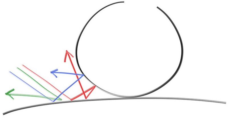
Figure 9: Light ray bounces

They might also be absorbed rather than reflected. The darker the surface, the more likely the ray is absorbed (that’s why it’s dark!). Really any algorithm that randomizes direction will produce surfaces that look matte. Let’s start with the most intuitive: a surface that randomly bounces a ray equally in all directions. For this material, a ray that hits the surface has an equal probability of bouncing in any direction away from the surface.

 

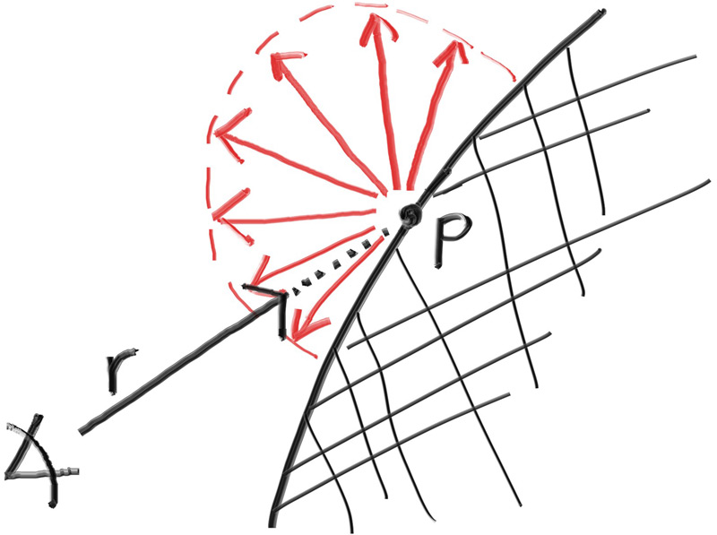
Figure 10: Equal reflection above the horizon

This very intuitive material is the simplest kind of diffuse and — indeed — many of the first raytracing papers used this diffuse method (before adopting a more accurate method that we’ll be implementing a little bit later). We don’t currently have a way to randomly reflect a ray, so we’ll need to add a few functions to our vector utility header. The first thing we need is the ability to generate arbitrary random vectors:

 

class vec3 {
  public:
    ...
 
    double length_squared() const {
        return e[0]*e[0] + e[1]*e[1] + e[2]*e[2];
    }
 
    static vec3 random() {
        return vec3(random_double(), random_double(), random_double());
    }
 
    static vec3 random(double min, double max) {
        return vec3(random_double(min,max), random_double(min,max), random_double(min,max));
    }};

Listing 47: [vec3.h] vec3 random utility functions

Then we need to figure out how to manipulate a random vector so that we only get results that are on the surface of a hemisphere. There are analytical methods of doing this, but they are actually surprisingly complicated to understand, and quite a bit complicated to implement. Instead, we’ll use what is typically the easiest algorithm: A rejection method. A rejection method works by repeatedly generating random samples until we produce a sample that meets the desired criteria. In other words, keep rejecting bad samples until you find a good one.

There are many equally valid ways of generating a random vector on a hemisphere using the rejection method, but for our purposes we will go with the simplest, which is:

1. Generate a random vector inside the unit sphere
2. Normalize this vector to extend it to the sphere surface
3. Invert the normalized vector if it falls onto the wrong hemisphere

First, we will use a rejection method to generate the random vector inside the unit sphere (that is, a sphere of radius 1). Pick a random point inside the cube enclosing the unit sphere (that is, where $x$, $y$, and $z$ are all in the range $[-1,+1]$). If this point lies outside the unit sphere, then generate a new one until we find one that lies inside or on the unit sphere.

 

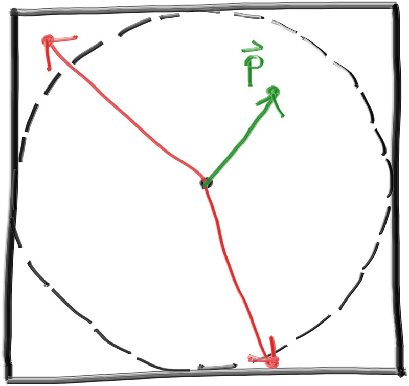
Figure 11: Two vectors were rejected before finding a good one (pre-normalization)

 

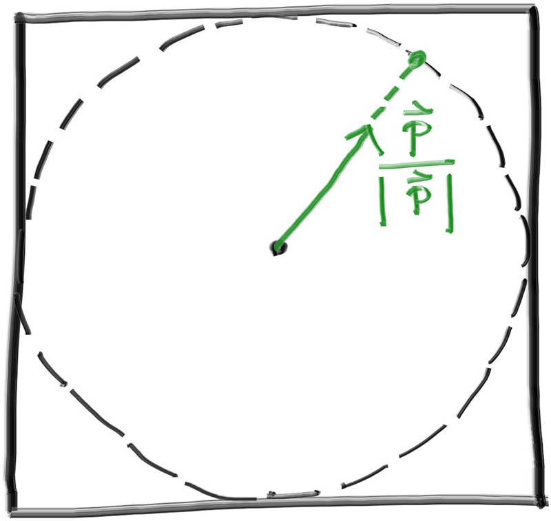
Figure 12: The accepted random vector is normalized to produce a unit vector

Here’s our first draft of the function:

...
 
inline vec3 unit_vector(const vec3& v) {
    return v / v.length();
}
 
inline vec3 random_unit_vector() {
    while (true) {
        auto p = vec3::random(-1,1);
        auto lensq = p.length_squared();
        if (lensq <= 1)
            return p / sqrt(lensq);
    }
}

Listing 48: [vec3.h] The random_unit_vector() function, version one

Sadly, we have a small floating-point abstraction leak to deal with. Since floating-point numbers have finite precision, a very small value can underflow to zero when squared. So if all three coordinates are small enough (that is, very near the center of the sphere), the norm of the vector will be zero, and thus normalizing will yield the bogus vector $[\pm \infty ,\pm \infty ,\pm \infty ]$. To fix this, we’ll also reject points that lie inside this “black hole” around the center. With double precision (64-bit floats), we can safely support values greater than ${\left(10\right)}^{-160}$.

Here’s our more robust function:

 

inline vec3 random_unit_vector() {
    while (true) {
        auto p = vec3::random(-1,1);
        auto lensq = p.length_squared();        if (1e-160 < lensq && lensq <= 1)            return p / sqrt(lensq);
    }
}

Listing 49: [vec3.h] The random_unit_vector() function, version one

Now that we have a random vector on the surface of the unit sphere, we can determine if it is on the correct hemisphere by comparing against the surface normal:

 

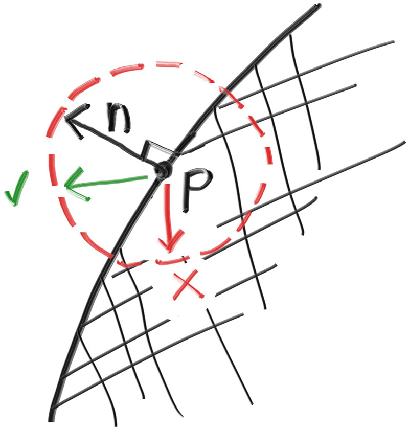
Figure 13: The normal vector tells us which hemisphere we need

We can take the dot product of the surface normal and our random vector to determine if it’s in the correct hemisphere. If the dot product is positive, then the vector is in the correct hemisphere. If the dot product is negative, then we need to invert the vector.

...
 
inline vec3 random_unit_vector() {
    while (true) {
        auto p = vec3::random(-1,1);
        auto lensq = p.length_squared();
        if (1e-160 < lensq && lensq <= 1)
            return p / sqrt(lensq);
    }
}
 
inline vec3 random_on_hemisphere(const vec3& normal) {
    vec3 on_unit_sphere = random_unit_vector();
    if (dot(on_unit_sphere, normal) > 0.0) // In the same hemisphere as the normal
        return on_unit_sphere;
    else
        return -on_unit_sphere;
}

Listing 50: [vec3.h] The random_on_hemisphere() function

If a ray bounces off of a material and keeps 100% of its color, then we say that the material is white. If a ray bounces off of a material and keeps 0% of its color, then we say that the material is black. As a first demonstration of our new diffuse material we’ll set the ray_color function to return 50% of the color from a bounce. We should expect to get a nice gray color.

 

class camera {
  ...
  private:
    ...
    color ray_color(const ray& r, const hittable& world) const {
        hit_record rec;
 
        if (world.hit(r, interval(0, infinity), rec)) {            vec3 direction = random_on_hemisphere(rec.normal);
            return 0.5 * ray_color(ray(rec.p, direction), world);        }
 
        vec3 unit_direction = unit_vector(r.direction());
        auto a = 0.5*(unit_direction.y() + 1.0);
        return (1.0-a)*color(1.0, 1.0, 1.0) + a*color(0.5, 0.7, 1.0);
    }
};

Listing 51: [camera.h] ray_color() using a random ray direction

… Indeed we do get rather nice gray spheres:

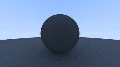
Image 7: First render of a diffuse sphere

   

Limiting the Number of Child Rays

There’s one potential problem lurking here. Notice that the ray_color function is recursive. When will it stop recursing? When it fails to hit anything. In some cases, however, that may be a long time — long enough to blow the stack. To guard against that, let’s limit the maximum recursion depth, returning no light contribution at the maximum depth:

 

class camera {
  public:
    double aspect_ratio      = 1.0;  // Ratio of image width over height
    int    image_width       = 100;  // Rendered image width in pixel count
    int    samples_per_pixel = 10;   // Count of random samples for each pixel    int    max_depth         = 10;   // Maximum number of ray bounces into scene
    void render(const hittable& world) {
        initialize();
 
        std::cout << "P3\n" << image_width << ' ' << image_height << "\n255\n";
 
        for (int j = 0; j < image_height; j++) {
            std::clog << "\rScanlines remaining: " << (image_height - j) << ' ' << std::flush;
            for (int i = 0; i < image_width; i++) {
                color pixel_color(0,0,0);
                for (int sample = 0; sample < samples_per_pixel; sample++) {
                    ray r = get_ray(i, j);                    pixel_color += ray_color(r, max_depth, world);                }
                write_color(std::cout, pixel_samples_scale * pixel_color);
            }
        }
 
        std::clog << "\rDone.                 \n";
    }
    ...
  private:
    ...    color ray_color(const ray& r, int depth, const hittable& world) const {
        // If we've exceeded the ray bounce limit, no more light is gathered.
        if (depth <= 0)
            return color(0,0,0);
        hit_record rec;
 
        if (world.hit(r, interval(0, infinity), rec)) {
            vec3 direction = random_on_hemisphere(rec.normal);            return 0.5 * ray_color(ray(rec.p, direction), depth-1, world);        }
 
        vec3 unit_direction = unit_vector(r.direction());
        auto a = 0.5*(unit_direction.y() + 1.0);
        return (1.0-a)*color(1.0, 1.0, 1.0) + a*color(0.5, 0.7, 1.0);
    }
};

Listing 52: [camera.h] camera::ray_color() with depth limiting

Update the main() function to use this new depth limit:

int main() {
    ...
 
    camera cam;
 
    cam.aspect_ratio      = 16.0 / 9.0;
    cam.image_width       = 400;
    cam.samples_per_pixel = 100;    cam.max_depth         = 50;
    cam.render(world);
}

Listing 53: [main.cc] Using the new ray depth limiting

For this very simple scene we should get basically the same result:

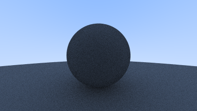
Image 8: Second render of a diffuse sphere with limited bounces

   

Fixing Shadow Acne

There’s also a subtle bug that we need to address. A ray will attempt to accurately calculate the intersection point when it intersects with a surface. Unfortunately for us, this calculation is susceptible to floating point rounding errors which can cause the intersection point to be ever so slightly off. This means that the origin of the next ray, the ray that is randomly scattered off of the surface, is unlikely to be perfectly flush with the surface. It might be just above the surface. It might be just below the surface. If the ray’s origin is just below the surface then it could intersect with that surface again. Which means that it will find the nearest surface at $t=0.00000001$ or whatever floating point approximation the hit function gives us. The simplest hack to address this is just to ignore hits that are very close to the calculated intersection point:

 

class camera {
  ...
  private:
    ...
    color ray_color(const ray& r, int depth, const hittable& world) const {
        // If we've exceeded the ray bounce limit, no more light is gathered.
        if (depth <= 0)
            return color(0,0,0);
 
        hit_record rec;
 
        if (world.hit(r, interval(0.001, infinity), rec)) {            vec3 direction = random_on_hemisphere(rec.normal);
            return 0.5 * ray_color(ray(rec.p, direction), depth-1, world);
        }
 
        vec3 unit_direction = unit_vector(r.direction());
        auto a = 0.5*(unit_direction.y() + 1.0);
        return (1.0-a)*color(1.0, 1.0, 1.0) + a*color(0.5, 0.7, 1.0);
    }
};

Listing 54: [camera.h] Calculating reflected ray origins with tolerance

This gets rid of the shadow acne problem. Yes it is really called that. Here’s the result:

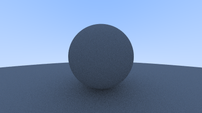
Image 9: Diffuse sphere with no shadow acne

   

True Lambertian Reflection

Scattering reflected rays evenly about the hemisphere produces a nice soft diffuse model, but we can definitely do better. A more accurate representation of real diffuse objects is the Lambertian distribution. This distribution scatters reflected rays in a manner that is proportional to $cos(\varphi )$, where $\varphi$ is the angle between the reflected ray and the surface normal. This means that a reflected ray is most likely to scatter in a direction near the surface normal, and less likely to scatter in directions away from the normal. This non-uniform Lambertian distribution does a better job of modeling material reflection in the real world than our previous uniform scattering.

We can create this distribution by adding a random unit vector to the normal vector. At the point of intersection on a surface there is the hit point, $\mathbf{p}$, and there is the normal of the surface, $\mathbf{n}$. At the point of intersection, this surface has exactly two sides, so there can only be two unique unit spheres tangent to any intersection point (one unique sphere for each side of the surface). These two unit spheres will be displaced from the surface by the length of their radius, which is exactly one for a unit sphere.

One sphere will be displaced in the direction of the surface’s normal ($\mathbf{n}$) and one sphere will be displaced in the opposite direction ($-\mathbf{n}$). This leaves us with two spheres of unit size that will only be just touching the surface at the intersection point. From this, one of the spheres will have its center at $(\mathbf{P}+\mathbf{n})$ and the other sphere will have its center at $(\mathbf{P}-\mathbf{n})$. The sphere with a center at $(\mathbf{P}-\mathbf{n})$ is considered inside the surface, whereas the sphere with center $(\mathbf{P}+\mathbf{n})$ is considered outside the surface.

We want to select the tangent unit sphere that is on the same side of the surface as the ray origin. Pick a random point $\mathbf{S}$ on this unit radius sphere and send a ray from the hit point $\mathbf{P}$ to the random point $\mathbf{S}$ (this is the vector $(\mathbf{S}-\mathbf{P})$):

 

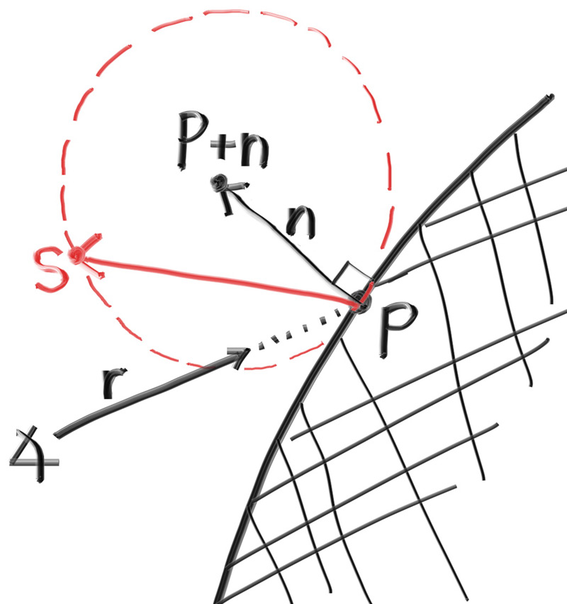
Figure 14: Randomly generating a vector according to Lambertian distribution

The change is actually fairly minimal:

class camera {
    ...
    color ray_color(const ray& r, int depth, const hittable& world) const {
        // If we've exceeded the ray bounce limit, no more light is gathered.
        if (depth <= 0)
            return color(0,0,0);
 
        hit_record rec;
 
        if (world.hit(r, interval(0.001, infinity), rec)) {            vec3 direction = rec.normal + random_unit_vector();            return 0.5 * ray_color(ray(rec.p, direction), depth-1, world);
        }
 
        vec3 unit_direction = unit_vector(r.direction());
        auto a = 0.5*(unit_direction.y() + 1.0);
        return (1.0-a)*color(1.0, 1.0, 1.0) + a*color(0.5, 0.7, 1.0);
    }
};

Listing 55: [camera.h] ray_color() with replacement diffuse

After rendering we get a similar image:

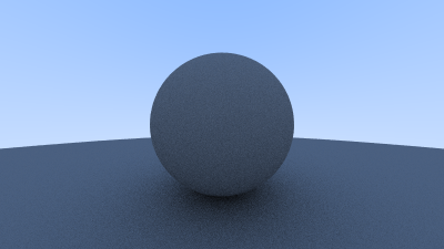
Image 10: Correct rendering of Lambertian spheres

It’s hard to tell the difference between these two diffuse methods, given that our scene of two spheres is so simple, but you should be able to notice two important visual differences:

1. The shadows are more pronounced after the change
2. Both spheres are tinted blue from the sky after the change

Both of these changes are due to the less uniform scattering of the light rays—more rays are scattering toward the normal. This means that for diffuse objects, they will appear darker because less light bounces toward the camera. For the shadows, more light bounces straight-up, so the area underneath the sphere is darker.

Not a lot of common, everyday objects are perfectly diffuse, so our visual intuition of how these objects behave under light can be poorly formed. As scenes become more complicated over the course of the book, you are encouraged to switch between the different diffuse renderers presented here. Most scenes of interest will contain a large amount of diffuse materials. You can gain valuable insight by understanding the effect of different diffuse methods on the lighting of a scene.

   

Using Gamma Correction for Accurate Color Intensity

Note the shadowing under the sphere. The picture is very dark, but our spheres only absorb half the energy of each bounce, so they are 50% reflectors. The spheres should look pretty bright (in real life, a light grey) but they appear to be rather dark. We can see this more clearly if we walk through the full brightness gamut for our diffuse material. We start by setting the reflectance of the ray_color function from 0.5 (50%) to 0.1 (10%):

 

class camera {
    ...
    color ray_color(const ray& r, int depth, const hittable& world) const {
        // If we've exceeded the ray bounce limit, no more light is gathered.
        if (depth <= 0)
            return color(0,0,0);
 
        hit_record rec;
 
        if (world.hit(r, interval(0.001, infinity), rec)) {
            vec3 direction = rec.normal + random_unit_vector();            return 0.1 * ray_color(ray(rec.p, direction), depth-1, world);        }
 
        vec3 unit_direction = unit_vector(r.direction());
        auto a = 0.5*(unit_direction.y() + 1.0);
        return (1.0-a)*color(1.0, 1.0, 1.0) + a*color(0.5, 0.7, 1.0);
    }
};

Listing 56: [camera.h] ray_color() with 10% reflectance

We render out at this new 10% reflectance. We then set reflectance to 30% and render again. We repeat for 50%, 70%, and finally 90%. You can overlay these images from left to right in the photo editor of your choice and you should get a very nice visual representation of the increasing brightness of your chosen gamut. This is the one that we’ve been working with so far:

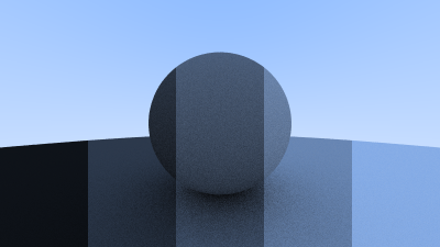
Image 11: The gamut of our renderer so far

If you look closely, or if you use a color picker, you should notice that the 50% reflectance render (the one in the middle) is far too dark to be half-way between white and black (middle-gray). Indeed, the 70% reflector is closer to middle-gray. The reason for this is that almost all computer programs assume that an image is “gamma corrected” before being written into an image file. This means that the 0 to 1 values have some transform applied before being stored as a byte. Images with data that are written without being transformed are said to be in linear space, whereas images that are transformed are said to be in gamma space. It is likely that the image viewer you are using is expecting an image in gamma space, but we are giving it an image in linear space. This is the reason why our image appears inaccurately dark.

There are many good reasons for why images should be stored in gamma space, but for our purposes we just need to be aware of it. We are going to transform our data into gamma space so that our image viewer can more accurately display our image. As a simple approximation, we can use “gamma 2” as our transform, which is the power that you use when going from gamma space to linear space. We need to go from linear space to gamma space, which means taking the inverse of “gamma 2”, which means an exponent of $1/gamma$, which is just the square-root. We’ll also want to ensure that we robustly handle negative inputs.

 

inline double linear_to_gamma(double linear_component)
{
    if (linear_component > 0)
        return std::sqrt(linear_component);
 
    return 0;
}
void write_color(std::ostream& out, const color& pixel_color) {
    auto r = pixel_color.x();
    auto g = pixel_color.y();
    auto b = pixel_color.z();
 
    // Apply a linear to gamma transform for gamma 2
    r = linear_to_gamma(r);
    g = linear_to_gamma(g);
    b = linear_to_gamma(b);
    // Translate the [0,1] component values to the byte range [0,255].
    static const interval intensity(0.000, 0.999);
    int rbyte = int(256 * intensity.clamp(r));
    int gbyte = int(256 * intensity.clamp(g));
    int bbyte = int(256 * intensity.clamp(b));
 
    // Write out the pixel color components.
    out << rbyte << ' ' << gbyte << ' ' << bbyte << '\n';
}

Listing 57: [color.h] write_color(), with gamma correction

Using this gamma correction, we now get a much more consistent ramp from darkness to lightness:

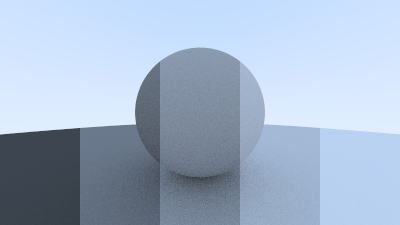
Image 12: The gamut of our renderer, gamma-corrected

   

Metal

   

An Abstract Class for Materials

If we want different objects to have different materials, we have a design decision. We could have a universal material type with lots of parameters so any individual material type could just ignore the parameters that don’t affect it. This is not a bad approach. Or we could have an abstract material class that encapsulates unique behavior. I am a fan of the latter approach. For our program the material needs to do two things:

1. Produce a scattered ray (or say it absorbed the incident ray).
2. If scattered, say how much the ray should be attenuated.

This suggests the abstract class:

#ifndef MATERIAL_H
#define MATERIAL_H
 
#include "hittable.h"
 
class material {
  public:
    virtual ~material() = default;
 
    virtual bool scatter(
        const ray& r_in, const hit_record& rec, color& attenuation, ray& scattered
    ) const {
        return false;
    }
};
 
#endif

Listing 58: [material.h] The material class

   

A Data Structure to Describe Ray-Object Intersections

The hit_record is to avoid a bunch of arguments so we can stuff whatever info we want in there. You can use arguments instead of an encapsulated type, it’s just a matter of taste. Hittables and materials need to be able to reference the other’s type in code so there is some circularity of the references. In C++ we add the line class material; to tell the compiler that material is a class that will be defined later. Since we’re just specifying a pointer to the class, the compiler doesn’t need to know the details of the class, solving the circular reference issue.

 

class material;
class hit_record {
  public:
    point3 p;
    vec3 normal;    shared_ptr<material> mat;    double t;
    bool front_face;
 
    void set_face_normal(const ray& r, const vec3& outward_normal) {
        front_face = dot(r.direction(), outward_normal) < 0;
        normal = front_face ? outward_normal : -outward_normal;
    }
};

Listing 59: [hittable.h] Hit record with added material pointer

hit_record is just a way to stuff a bunch of arguments into a class so we can send them as a group. When a ray hits a surface (a particular sphere for example), the material pointer in the hit_record will be set to point at the material pointer the sphere was given when it was set up in main() when we start. When the ray_color() routine gets the hit_record it can call member functions of the material pointer to find out what ray, if any, is scattered.

To achieve this, hit_record needs to be told the material that is assigned to the sphere.

class sphere : public hittable {
  public:    sphere(const point3& center, double radius) : center(center), radius(std::fmax(0,radius)) {
        // TODO: Initialize the material pointer \`mat\`.
    }
    bool hit(const ray& r, interval ray_t, hit_record& rec) const override {
        ...
 
        rec.t = root;
        rec.p = r.at(rec.t);
        vec3 outward_normal = (rec.p - center) / radius;
        rec.set_face_normal(r, outward_normal);        rec.mat = mat;
        return true;
    }
 
  private:
    point3 center;
    double radius;    shared_ptr<material> mat;};

Listing 60: [sphere.h] Ray-sphere intersection with added material information

   

Modeling Light Scatter and Reflectance

Here and throughout these books we will use the term albedo (Latin for “whiteness”). Albedo is a precise technical term in some disciplines, but in all cases it is used to define some form of fractional reflectance. Albedo will vary with material color and (as we will later implement for glass materials) can also vary with incident viewing direction (the direction of the incoming ray).

Lambertian (diffuse) reflectance can either always scatter and attenuate light according to its reflectance $R$, or it can sometimes scatter (with probability $1-R$) with no attenuation (where a ray that isn’t scattered is just absorbed into the material). It could also be a mixture of both those strategies. We will choose to always scatter, so implementing Lambertian materials becomes a simple task:

 

class material {
    ...
};
 
class lambertian : public material {
  public:
    lambertian(const color& albedo) : albedo(albedo) {}
 
    bool scatter(const ray& r_in, const hit_record& rec, color& attenuation, ray& scattered)
    const override {
        auto scatter_direction = rec.normal + random_unit_vector();
        scattered = ray(rec.p, scatter_direction);
        attenuation = albedo;
        return true;
    }
 
  private:
    color albedo;
};

Listing 61: [material.h] The new lambertian material class

Note the third option: we could scatter with some fixed probability $p$ and have attenuation be $albedo/p$. Your choice.

If you read the code above carefully, you’ll notice a small chance of mischief. If the random unit vector we generate is exactly opposite the normal vector, the two will sum to zero, which will result in a zero scatter direction vector. This leads to bad scenarios later on (infinities and NaNs), so we need to intercept the condition before we pass it on.

In service of this, we’ll create a new vector method — vec3::near_zero() — that returns true if the vector is very close to zero in all dimensions.

The following changes will use the C++ standard library function std::fabs, which returns the absolute value of its input.

 

class vec3 {
    ...
 
    double length_squared() const {
        return e[0]*e[0] + e[1]*e[1] + e[2]*e[2];
    }
 
    bool near_zero() const {
        // Return true if the vector is close to zero in all dimensions.
        auto s = 1e-8;
        return (std::fabs(e[0]) < s) && (std::fabs(e[1]) < s) && (std::fabs(e[2]) < s);
    }
    ...
};

Listing 62: [vec3.h] The vec3::near_zero() method

 

class lambertian : public material {
  public:
    lambertian(const color& albedo) : albedo(albedo) {}
 
    bool scatter(const ray& r_in, const hit_record& rec, color& attenuation, ray& scattered)
    const override {
        auto scatter_direction = rec.normal + random_unit_vector();
 
        // Catch degenerate scatter direction
        if (scatter_direction.near_zero())
            scatter_direction = rec.normal;
        scattered = ray(rec.p, scatter_direction);
        attenuation = albedo;
        return true;
    }
 
  private:
    color albedo;
};

Listing 63: [material.h] Lambertian scatter, bullet-proof

   

Mirrored Light Reflection

For polished metals the ray won’t be randomly scattered. The key question is: How does a ray get reflected from a metal mirror? Vector math is our friend here:

 

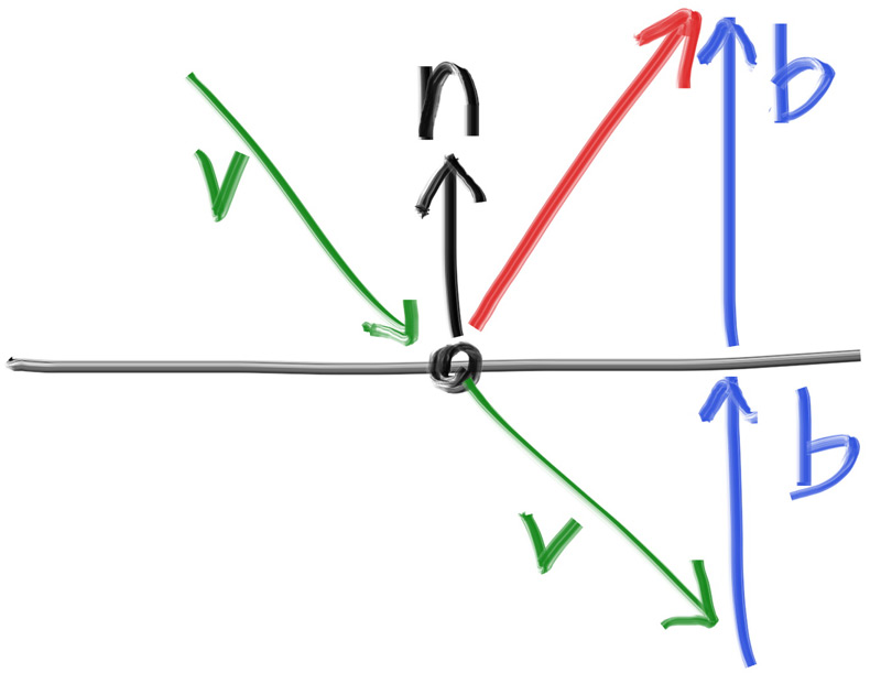
Figure 15: Ray reflection

The reflected ray direction in red is just $\mathbf{v}+2\mathbf{b}$. In our design, $\mathbf{n}$ is a unit vector (length one), but $\mathbf{v}$ may not be. To get the vector $\mathbf{b}$, we scale the normal vector by the length of the projection of $\mathbf{v}$ onto $\mathbf{n}$, which is given by the dot product $\mathbf{v}\cdot \mathbf{n}$. (If $\mathbf{n}$ were not a unit vector, we would also need to divide this dot product by the length of $\mathbf{n}$.) Finally, because $\mathbf{v}$ points into the surface, and we want $\mathbf{b}$ to point out of the surface, we need to negate this projection length.

Putting everything together, we get the following computation of the reflected vector:

 

...
 
inline vec3 random_on_hemisphere(const vec3& normal) {
    ...
}
 
inline vec3 reflect(const vec3& v, const vec3& n) {
    return v - 2*dot(v,n)*n;
}

Listing 64: [vec3.h] vec3 reflection function

The metal material just reflects rays using that formula:

...
 
class lambertian : public material {
    ...
};
 
class metal : public material {
  public:
    metal(const color& albedo) : albedo(albedo) {}
 
    bool scatter(const ray& r_in, const hit_record& rec, color& attenuation, ray& scattered)
    const override {
        vec3 reflected = reflect(r_in.direction(), rec.normal);
        scattered = ray(rec.p, reflected);
        attenuation = albedo;
        return true;
    }
 
  private:
    color albedo;
};

Listing 65: [material.h] Metal material with reflectance function

We need to modify the ray_color() function for all of our changes:

#include "hittable.h"#include "material.h"...
 
class camera {
  ...
  private:
    ...
    color ray_color(const ray& r, int depth, const hittable& world) const {
        // If we've exceeded the ray bounce limit, no more light is gathered.
        if (depth <= 0)
            return color(0,0,0);
 
        hit_record rec;
 
        if (world.hit(r, interval(0.001, infinity), rec)) {            ray scattered;
            color attenuation;
            if (rec.mat->scatter(r, rec, attenuation, scattered))
                return attenuation * ray_color(scattered, depth-1, world);
            return color(0,0,0);        }
 
        vec3 unit_direction = unit_vector(r.direction());
        auto a = 0.5*(unit_direction.y() + 1.0);
        return (1.0-a)*color(1.0, 1.0, 1.0) + a*color(0.5, 0.7, 1.0);
    }
};

Listing 66: [camera.h] Ray color with scattered reflectance

Now we’ll update the sphere constructor to initialize the material pointer mat:

 

class sphere : public hittable {
  public:    sphere(const point3& center, double radius, shared_ptr<material> mat)
      : center(center), radius(std::fmax(0,radius)), mat(mat) {}
    ...
};

Listing 67: [sphere.h] Initializing sphere with a material

   

A Scene with Metal Spheres

Now let’s add some metal spheres to our scene:

 

#include "rtweekend.h"
 
#include "camera.h"
#include "hittable.h"
#include "hittable_list.h"#include "material.h"#include "sphere.h"
 
int main() {
    hittable_list world;
 
    auto material_ground = make_shared<lambertian>(color(0.8, 0.8, 0.0));
    auto material_center = make_shared<lambertian>(color(0.1, 0.2, 0.5));
    auto material_left   = make_shared<metal>(color(0.8, 0.8, 0.8));
    auto material_right  = make_shared<metal>(color(0.8, 0.6, 0.2));
 
    world.add(make_shared<sphere>(point3( 0.0, -100.5, -1.0), 100.0, material_ground));
    world.add(make_shared<sphere>(point3( 0.0,    0.0, -1.2),   0.5, material_center));
    world.add(make_shared<sphere>(point3(-1.0,    0.0, -1.0),   0.5, material_left));
    world.add(make_shared<sphere>(point3( 1.0,    0.0, -1.0),   0.5, material_right));
    camera cam;
 
    cam.aspect_ratio      = 16.0 / 9.0;
    cam.image_width       = 400;
    cam.samples_per_pixel = 100;
    cam.max_depth         = 50;
 
    cam.render(world);
}

Listing 68: [main.cc] Scene with metal spheres

Which gives:

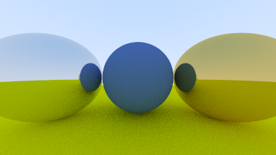
Image 13: Shiny metal

   

Fuzzy Reflection

We can also randomize the reflected direction by using a small sphere and choosing a new endpoint for the ray. We’ll use a random point from the surface of a sphere centered on the original endpoint, scaled by the fuzz factor.

 

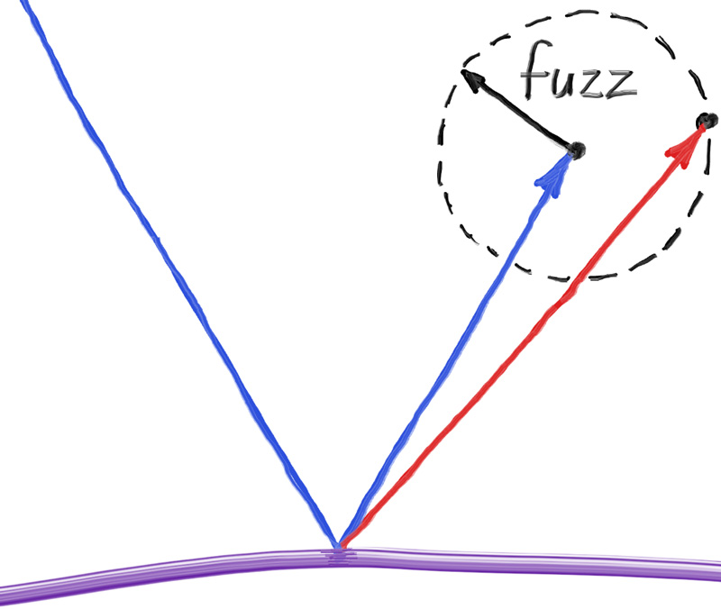
Figure 16: Generating fuzzed reflection rays

The bigger the fuzz sphere, the fuzzier the reflections will be. This suggests adding a fuzziness parameter that is just the radius of the sphere (so zero is no perturbation). The catch is that for big spheres or grazing rays, we may scatter below the surface. We can just have the surface absorb those.

Also note that in order for the fuzz sphere to make sense, it needs to be consistently scaled compared to the reflection vector, which can vary in length arbitrarily. To address this, we need to normalize the reflected ray.

 

class metal : public material {
  public:    metal(const color& albedo, double fuzz) : albedo(albedo), fuzz(fuzz < 1 ? fuzz : 1) {}
    bool scatter(const ray& r_in, const hit_record& rec, color& attenuation, ray& scattered)
    const override {
        vec3 reflected = reflect(r_in.direction(), rec.normal);        reflected = unit_vector(reflected) + (fuzz * random_unit_vector());        scattered = ray(rec.p, reflected);
        attenuation = albedo;        return (dot(scattered.direction(), rec.normal) > 0);    }
 
  private:
    color albedo;    double fuzz;};

Listing 69: [material.h] Metal material fuzziness

We can try that out by adding fuzziness 0.3 and 1.0 to the metals:

int main() {
    ...
    auto material_ground = make_shared<lambertian>(color(0.8, 0.8, 0.0));
    auto material_center = make_shared<lambertian>(color(0.1, 0.2, 0.5));    auto material_left   = make_shared<metal>(color(0.8, 0.8, 0.8), 0.3);
    auto material_right  = make_shared<metal>(color(0.8, 0.6, 0.2), 1.0);    ...
}

Listing 70: [main.cc] Metal spheres with fuzziness

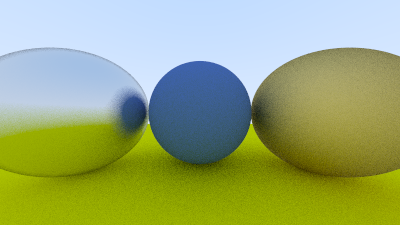
Image 14: Fuzzed metal

   

Dielectrics

Clear materials such as water, glass, and diamond are dielectrics. When a light ray hits them, it splits into a reflected ray and a refracted (transmitted) ray. We’ll handle that by randomly choosing between reflection and refraction, only generating one scattered ray per interaction.

As a quick review of terms, a reflected ray hits a surface and then “bounces” off in a new direction.

A refracted ray bends as it transitions from a material’s surroundings into the material itself (as with glass or water). This is why a pencil looks bent when partially inserted in water.

The amount that a refracted ray bends is determined by the material’s refractive index. Generally, this is a single value that describes how much light bends when entering a material from a vacuum. Glass has a refractive index of something like 1.5–1.7, diamond is around 2.4, and air has a small refractive index of 1.000293.

When a transparent material is embedded in a different transparent material, you can describe the refraction with a relative refraction index: the refractive index of the object’s material divided by the refractive index of the surrounding material. For example, if you want to render a glass ball under water, then the glass ball would have an effective refractive index of 1.125. This is given by the refractive index of glass (1.5) divided by the refractive index of water (1.333).

You can find the refractive index of most common materials with a quick internet search.

   

Refraction

The hardest part to debug is the refracted ray. I usually first just have all the light refract if there is a refraction ray at all. For this project, I tried to put two glass balls in our scene, and I got this (I have not told you how to do this right or wrong yet, but soon!):

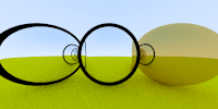
Image 15: Glass first

Is that right? Glass balls look odd in real life. But no, it isn’t right. The world should be flipped upside down and no weird black stuff. I just printed out the ray straight through the middle of the image and it was clearly wrong. That often does the job.

   

Snell’s Law

The refraction is described by Snell’s law:

$$\eta \cdot sin\theta ={\left(\eta \right)}^{{}^{\prime }}\cdot sin{\left(\theta \right)}^{{}^{\prime }}$$

Where $\theta$ and ${\left(\theta \right)}^{{}^{\prime }}$ are the angles from the normal, and $\eta$ and ${\left(\eta \right)}^{{}^{\prime }}$ (pronounced “eta” and “eta prime”) are the refractive indices. The geometry is:

 

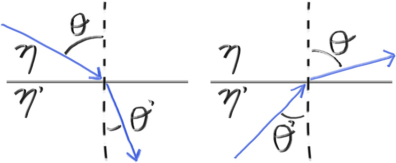
Figure 17: Ray refraction

In order to determine the direction of the refracted ray, we have to solve for $sin{\left(\theta \right)}^{{}^{\prime }}$:

$$sin{\left(\theta \right)}^{{}^{\prime }}=\frac{\eta }{{\left(\eta \right)}^{{}^{\prime }}}\cdot sin\theta$$

On the refracted side of the surface there is a refracted ray ${\left(\mathbf{R}\right)}^{{}^{\prime }}$ and a normal ${\left(\mathbf{n}\right)}^{{}^{\prime }}$, and there exists an angle, ${\left(\theta \right)}^{{}^{\prime }}$, between them. We can split ${\left(\mathbf{R}\right)}^{{}^{\prime }}$ into the parts of the ray that are perpendicular to ${\left(\mathbf{n}\right)}^{{}^{\prime }}$ and parallel to ${\left(\mathbf{n}\right)}^{{}^{\prime }}$:

$${\left(\mathbf{R}\right)}^{{}^{\prime }}={\left({\left(\mathbf{R}\right)}^{{}^{\prime }}\right)}_{\perp }+{\left({\left(\mathbf{R}\right)}^{{}^{\prime }}\right)}_{\parallel }$$

If we solve for ${\left({\left(\mathbf{R}\right)}^{{}^{\prime }}\right)}_{\perp }$ and ${\left({\left(\mathbf{R}\right)}^{{}^{\prime }}\right)}_{\parallel }$ we get:

$${\left({\left(\mathbf{R}\right)}^{{}^{\prime }}\right)}_{\perp }=\frac{\eta }{{\left(\eta \right)}^{{}^{\prime }}}(\mathbf{R}+cos\theta \mathbf{n})$$ $${\left({\left(\mathbf{R}\right)}^{{}^{\prime }}\right)}_{\parallel }=-\sqrt{1-|{\left({\left(\mathbf{R}\right)}^{{}^{\prime }}\right)}_{\perp }{\left(|\right)}^2}\mathbf{n}$$

You can go ahead and prove this for yourself if you want, but we will treat it as fact and move on. The rest of the book will not require you to understand the proof.

We know the value of every term on the right-hand side except for $cos\theta$. It is well known that the dot product of two vectors can be explained in terms of the cosine of the angle between them:

$$\mathbf{a}\cdot \mathbf{b}=|\mathbf{a}||\mathbf{b}|cos\theta$$

If we restrict $\mathbf{a}$ and $\mathbf{b}$ to be unit vectors:

$$\mathbf{a}\cdot \mathbf{b}=cos\theta$$

We can now rewrite ${\left({\left(\mathbf{R}\right)}^{{}^{\prime }}\right)}_{\perp }$ in terms of known quantities:

$${\left({\left(\mathbf{R}\right)}^{{}^{\prime }}\right)}_{\perp }=\frac{\eta }{{\left(\eta \right)}^{{}^{\prime }}}(\mathbf{R}+(-\mathbf{R}\cdot \mathbf{n})\mathbf{n})$$

When we combine them back together, we can write a function to calculate ${\left(\mathbf{R}\right)}^{{}^{\prime }}$:

...
 
inline vec3 reflect(const vec3& v, const vec3& n) {
    return v - 2*dot(v,n)*n;
}
 
inline vec3 refract(const vec3& uv, const vec3& n, double etai_over_etat) {
    auto cos_theta = std::fmin(dot(-uv, n), 1.0);
    vec3 r_out_perp =  etai_over_etat * (uv + cos_theta*n);
    vec3 r_out_parallel = -std::sqrt(std::fabs(1.0 - r_out_perp.length_squared())) * n;
    return r_out_perp + r_out_parallel;
}

Listing 71: [vec3.h] Refraction function

And the dielectric material that always refracts is:

...
 
class metal : public material {
    ...
};
 
class dielectric : public material {
  public:
    dielectric(double refraction_index) : refraction_index(refraction_index) {}
 
    bool scatter(const ray& r_in, const hit_record& rec, color& attenuation, ray& scattered)
    const override {
        attenuation = color(1.0, 1.0, 1.0);
        double ri = rec.front_face ? (1.0/refraction_index) : refraction_index;
 
        vec3 unit_direction = unit_vector(r_in.direction());
        vec3 refracted = refract(unit_direction, rec.normal, ri);
 
        scattered = ray(rec.p, refracted);
        return true;
    }
 
  private:
    // Refractive index in vacuum or air, or the ratio of the material's refractive index over
    // the refractive index of the enclosing media
    double refraction_index;
};

Listing 72: [material.h] Dielectric material class that always refracts

Now we’ll update the scene to illustrate refraction by changing the left sphere to glass, which has an index of refraction of approximately 1.5.

auto material_ground = make_shared<lambertian>(color(0.8, 0.8, 0.0));
auto material_center = make_shared<lambertian>(color(0.1, 0.2, 0.5));auto material_left   = make_shared<dielectric>(1.50);auto material_right  = make_shared<metal>(color(0.8, 0.6, 0.2), 1.0);

Listing 73: [main.cc] Changing the left sphere to glass

This gives us the following result:

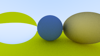
Image 16: Glass sphere that always refracts

   

Total Internal Reflection

One troublesome practical issue with refraction is that there are ray angles for which no solution is possible using Snell’s law. When a ray enters a medium of lower index of refraction at a sufficiently glancing angle, it can refract with an angle greater than 90°. If we refer back to Snell’s law and the derivation of $sin{\left(\theta \right)}^{{}^{\prime }}$:

$$sin{\left(\theta \right)}^{{}^{\prime }}=\frac{\eta }{{\left(\eta \right)}^{{}^{\prime }}}\cdot sin\theta$$

If the ray is inside glass and outside is air ($\eta =1.5$ and ${\left(\eta \right)}^{{}^{\prime }}=1.0$):

$$sin{\left(\theta \right)}^{{}^{\prime }}=\frac{1.5}{1.0}\cdot sin\theta$$

The value of $sin{\left(\theta \right)}^{{}^{\prime }}$ cannot be greater than 1. So, if,

$$\frac{1.5}{1.0}\cdot sin\theta >1.0$$

the equality between the two sides of the equation is broken, and a solution cannot exist. If a solution does not exist, the glass cannot refract, and therefore must reflect the ray:

if (ri * sin_theta > 1.0) {
    // Must Reflect
    ...
} else {
    // Can Refract
    ...
}

Listing 74: [material.h] Determining if the ray can refract

Here all the light is reflected, and because in practice that is usually inside solid objects, it is called total internal reflection. This is why sometimes the water-to-air boundary acts as a perfect mirror when you are submerged — if you’re under water looking up, you can see things above the water, but when you are close to the surface and looking sideways, the water surface looks like a mirror.

We can solve for sin_theta using the trigonometric qualities:

$$sin\theta =\sqrt{1-{\left(cos\right)}^2\theta }$$

and

$$cos\theta =\mathbf{R}\cdot \mathbf{n}$$

 

double cos_theta = std::fmin(dot(-unit_direction, rec.normal), 1.0);
double sin_theta = std::sqrt(1.0 - cos_theta*cos_theta);
 
if (ri * sin_theta > 1.0) {
    // Must Reflect
    ...
} else {
    // Can Refract
    ...
}

Listing 75: [material.h] Determining if the ray can refract

And the dielectric material that always refracts (when possible) is:

class dielectric : public material {
  public:
    dielectric(double refraction_index) : refraction_index(refraction_index) {}
 
    bool scatter(const ray& r_in, const hit_record& rec, color& attenuation, ray& scattered)
    const override {
        attenuation = color(1.0, 1.0, 1.0);
        double ri = rec.front_face ? (1.0/refraction_index) : refraction_index;
 
        vec3 unit_direction = unit_vector(r_in.direction());        double cos_theta = std::fmin(dot(-unit_direction, rec.normal), 1.0);
        double sin_theta = std::sqrt(1.0 - cos_theta*cos_theta);
 
        bool cannot_refract = ri * sin_theta > 1.0;
        vec3 direction;
 
        if (cannot_refract)
            direction = reflect(unit_direction, rec.normal);
        else
            direction = refract(unit_direction, rec.normal, ri);
 
        scattered = ray(rec.p, direction);        return true;
    }
 
  private:
    // Refractive index in vacuum or air, or the ratio of the material's refractive index over
    // the refractive index of the enclosing media
    double refraction_index;
};

Listing 76: [material.h] Dielectric material class with reflection

Attenuation is always 1 — the glass surface absorbs nothing.

If we render the prior scene with the new dielectric::scatter() function, we see … no change. Huh?

Well, it turns out that given a sphere of material with an index of refraction greater than air, there’s no incident angle that will yield total internal reflection — neither at the ray-sphere entrance point nor at the ray exit. This is due to the geometry of spheres, as a grazing incoming ray will always be bent to a smaller angle, and then bent back to the original angle on exit.

So how can we illustrate total internal reflection? Well, if the sphere has an index of refraction less than the medium it’s in, then we can hit it with shallow grazing angles, getting total external reflection. That should be good enough to observe the effect.

We’ll model a world filled with water (index of refraction approximately 1.33), and change the sphere material to air (index of refraction 1.00) — an air bubble! To do this, change the left sphere material’s index of refraction to

$$\frac{\text{index of refraction of air}}{\text{index of refraction of water}}$$

 

auto material_ground = make_shared<lambertian>(color(0.8, 0.8, 0.0));
auto material_center = make_shared<lambertian>(color(0.1, 0.2, 0.5));auto material_left   = make_shared<dielectric>(1.00 / 1.33);auto material_right  = make_shared<metal>(color(0.8, 0.6, 0.2), 1.0);

Listing 77: [main.cc] Left sphere is an air bubble in water

This change yields the following render:

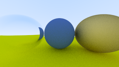
Image 17: Air bubble sometimes refracts, sometimes reflects

Here you can see that more-or-less direct rays refract, while glancing rays reflect.

   

Schlick Approximation

Now real glass has reflectivity that varies with angle — look at a window at a steep angle and it becomes a mirror. There is a big ugly equation for that, but almost everybody uses a cheap and surprisingly accurate polynomial approximation by Christophe Schlick. This yields our full glass material:

 

class dielectric : public material {
  public:
    dielectric(double refraction_index) : refraction_index(refraction_index) {}
 
    bool scatter(const ray& r_in, const hit_record& rec, color& attenuation, ray& scattered)
    const override {
        attenuation = color(1.0, 1.0, 1.0);
        double ri = rec.front_face ? (1.0/refraction_index) : refraction_index;
 
        vec3 unit_direction = unit_vector(r_in.direction());
        double cos_theta = std::fmin(dot(-unit_direction, rec.normal), 1.0);
        double sin_theta = std::sqrt(1.0 - cos_theta*cos_theta);
 
        bool cannot_refract = ri * sin_theta > 1.0;
        vec3 direction;
 
        if (cannot_refract || reflectance(cos_theta, ri) > random_double())            direction = reflect(unit_direction, rec.normal);
        else
            direction = refract(unit_direction, rec.normal, ri);
 
        scattered = ray(rec.p, direction);
        return true;
    }
 
  private:
    // Refractive index in vacuum or air, or the ratio of the material's refractive index over
    // the refractive index of the enclosing media
    double refraction_index;
 
    static double reflectance(double cosine, double refraction_index) {
        // Use Schlick's approximation for reflectance.
        auto r0 = (1 - refraction_index) / (1 + refraction_index);
        r0 = r0*r0;
        return r0 + (1-r0)*std::pow((1 - cosine),5);
    }};

Listing 78: [material.h] Full glass material

   

Modeling a Hollow Glass Sphere

Let’s model a hollow glass sphere. This is a sphere of some thickness with another sphere of air inside it. If you think about the path of a ray going through such an object, it will hit the outer sphere, refract, hit the inner sphere (assuming we do hit it), refract a second time, and travel through the air inside. Then it will continue on, hit the inside surface of the inner sphere, refract back, then hit the inside surface of the outer sphere, and finally refract and exit back into the scene atmosphere.

The outer sphere is just modeled with a standard glass sphere, with a refractive index of around 1.50 (modeling a refraction from the outside air into glass). The inner sphere is a bit different because its refractive index should be relative to the material of the surrounding outer sphere, thus modeling a transition from glass into the inner air.

This is actually simple to specify, as the refraction_index parameter to the dielectric material can be interpreted as the ratio of the refractive index of the object divided by the refractive index of the enclosing medium. In this case, the inner sphere would have an refractive index of air (the inner sphere material) over the index of refraction of glass (the enclosing medium), or $1.00/1.50=0.67$.

Here’s the code:

 

...
auto material_ground = make_shared<lambertian>(color(0.8, 0.8, 0.0));
auto material_center = make_shared<lambertian>(color(0.1, 0.2, 0.5));auto material_left   = make_shared<dielectric>(1.50);
auto material_bubble = make_shared<dielectric>(1.00 / 1.50);auto material_right  = make_shared<metal>(color(0.8, 0.6, 0.2), 0.0);
 
world.add(make_shared<sphere>(point3( 0.0, -100.5, -1.0), 100.0, material_ground));
world.add(make_shared<sphere>(point3( 0.0,    0.0, -1.2),   0.5, material_center));
world.add(make_shared<sphere>(point3(-1.0,    0.0, -1.0),   0.5, material_left));world.add(make_shared<sphere>(point3(-1.0,    0.0, -1.0),   0.4, material_bubble));world.add(make_shared<sphere>(point3( 1.0,    0.0, -1.0),   0.5, material_right));
...

Listing 79: [main.cc] Scene with hollow glass sphere

And here’s the result:

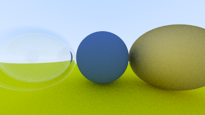
Image 18: A hollow glass sphere

   

Positionable Camera

Cameras, like dielectrics, are a pain to debug, so I always develop mine incrementally. First, let’s allow for an adjustable field of view (fov). This is the visual angle from edge to edge of the rendered image. Since our image is not square, the fov is different horizontally and vertically. I always use vertical fov. I also usually specify it in degrees and change to radians inside a constructor — a matter of personal taste.

   

Camera Viewing Geometry

First, we’ll keep the rays coming from the origin and heading to the $z=-1$ plane. We could make it the $z=-2$ plane, or whatever, as long as we made $h$ a ratio to that distance. Here is our setup:

 

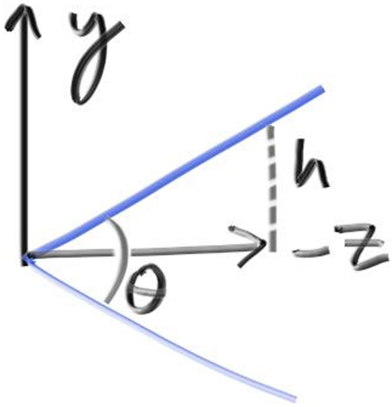
Figure 18: Camera viewing geometry (from the side)

This implies $h=tan(\frac{\theta }{2})$. Our camera now becomes:

class camera {
  public:
    double aspect_ratio      = 1.0;  // Ratio of image width over height
    int    image_width       = 100;  // Rendered image width in pixel count
    int    samples_per_pixel = 10;   // Count of random samples for each pixel
    int    max_depth         = 10;   // Maximum number of ray bounces into scene
 
    double vfov = 90;  // Vertical view angle (field of view)
    void render(const hittable& world) {
    ...
 
  private:
    ...
 
    void initialize() {
        image_height = int(image_width / aspect_ratio);
        image_height = (image_height < 1) ? 1 : image_height;
 
        pixel_samples_scale = 1.0 / samples_per_pixel;
 
        center = point3(0, 0, 0);
 
        // Determine viewport dimensions.
        auto focal_length = 1.0;        auto theta = degrees_to_radians(vfov);
        auto h = std::tan(theta/2);
        auto viewport_height = 2 * h * focal_length;        auto viewport_width = viewport_height * (double(image_width)/image_height);
 
        // Calculate the vectors across the horizontal and down the vertical viewport edges.
        auto viewport_u = vec3(viewport_width, 0, 0);
        auto viewport_v = vec3(0, -viewport_height, 0);
 
        // Calculate the horizontal and vertical delta vectors from pixel to pixel.
        pixel_delta_u = viewport_u / image_width;
        pixel_delta_v = viewport_v / image_height;
 
        // Calculate the location of the upper left pixel.
        auto viewport_upper_left =
            center - vec3(0, 0, focal_length) - viewport_u/2 - viewport_v/2;
        pixel00_loc = viewport_upper_left + 0.5 * (pixel_delta_u + pixel_delta_v);
    }
 
    ...
};

Listing 80: [camera.h] Camera with adjustable field-of-view (fov)

We’ll test out these changes with a simple scene of two touching spheres, using a 90° field of view.

int main() {
    hittable_list world;
 
    auto R = std::cos(pi/4);
 
    auto material_left  = make_shared<lambertian>(color(0,0,1));
    auto material_right = make_shared<lambertian>(color(1,0,0));
 
    world.add(make_shared<sphere>(point3(-R, 0, -1), R, material_left));
    world.add(make_shared<sphere>(point3( R, 0, -1), R, material_right));
    camera cam;
 
    cam.aspect_ratio      = 16.0 / 9.0;
    cam.image_width       = 400;
    cam.samples_per_pixel = 100;
    cam.max_depth         = 50;
 
    cam.vfov = 90;
    cam.render(world);
}

Listing 81: [main.cc] Scene with wide-angle camera

This gives us the rendering:

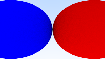
Image 19: A wide-angle view

   

Positioning and Orienting the Camera

To get an arbitrary viewpoint, let’s first name the points we care about. We’ll call the position where we place the camera lookfrom, and the point we look at lookat. (Later, if you want, you could define a direction to look in instead of a point to look at.)

We also need a way to specify the roll, or sideways tilt, of the camera: the rotation around the lookat-lookfrom axis. Another way to think about it is that even if you keep lookfrom and lookat constant, you can still rotate your head around your nose. What we need is a way to specify an “up” vector for the camera.

 

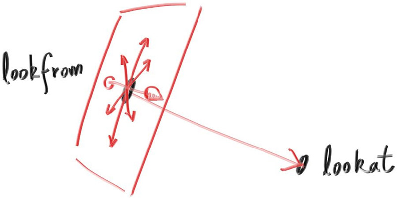
Figure 19: Camera view direction

We can specify any up vector we want, as long as it’s not parallel to the view direction. Project this up vector onto the plane orthogonal to the view direction to get a camera-relative up vector. I use the common convention of naming this the “view up” (vup) vector. After a few cross products and vector normalizations, we now have a complete orthonormal basis $(u,v,w)$ to describe our camera’s orientation. $u$ will be the unit vector pointing to camera right, $v$ is the unit vector pointing to camera up, $w$ is the unit vector pointing opposite the view direction (since we use right-hand coordinates), and the camera center is at the origin.

 

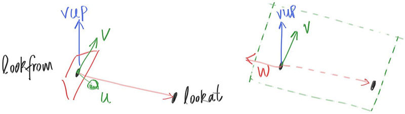
Figure 20: Camera view up direction

Like before, when our fixed camera faced $-Z$, our arbitrary view camera faces $-w$. Keep in mind that we can — but we don’t have to — use world up $(0,1,0)$ to specify vup. This is convenient and will naturally keep your camera horizontally level until you decide to experiment with crazy camera angles.

 

class camera {
  public:
    double aspect_ratio      = 1.0;  // Ratio of image width over height
    int    image_width       = 100;  // Rendered image width in pixel count
    int    samples_per_pixel = 10;   // Count of random samples for each pixel
    int    max_depth         = 10;   // Maximum number of ray bounces into scene
 
    double vfov     = 90;              // Vertical view angle (field of view)    point3 lookfrom = point3(0,0,0);   // Point camera is looking from
    point3 lookat   = point3(0,0,-1);  // Point camera is looking at
    vec3   vup      = vec3(0,1,0);     // Camera-relative "up" direction
    ...
 
  private:
    int    image_height;         // Rendered image height
    double pixel_samples_scale;  // Color scale factor for a sum of pixel samples
    point3 center;               // Camera center
    point3 pixel00_loc;          // Location of pixel 0, 0
    vec3   pixel_delta_u;        // Offset to pixel to the right
    vec3   pixel_delta_v;        // Offset to pixel below    vec3   u, v, w;              // Camera frame basis vectors
    void initialize() {
        image_height = int(image_width / aspect_ratio);
        image_height = (image_height < 1) ? 1 : image_height;
 
        pixel_samples_scale = 1.0 / samples_per_pixel;
 
        center = lookfrom;
        // Determine viewport dimensions.        auto focal_length = (lookfrom - lookat).length();        auto theta = degrees_to_radians(vfov);
        auto h = std::tan(theta/2);
        auto viewport_height = 2 * h * focal_length;
        auto viewport_width = viewport_height * (double(image_width)/image_height);
 
        // Calculate the u,v,w unit basis vectors for the camera coordinate frame.
        w = unit_vector(lookfrom - lookat);
        u = unit_vector(cross(vup, w));
        v = cross(w, u);
        // Calculate the vectors across the horizontal and down the vertical viewport edges.        vec3 viewport_u = viewport_width * u;    // Vector across viewport horizontal edge
        vec3 viewport_v = viewport_height * -v;  // Vector down viewport vertical edge
        // Calculate the horizontal and vertical delta vectors from pixel to pixel.
        pixel_delta_u = viewport_u / image_width;
        pixel_delta_v = viewport_v / image_height;
 
        // Calculate the location of the upper left pixel.        auto viewport_upper_left = center - (focal_length * w) - viewport_u/2 - viewport_v/2;        pixel00_loc = viewport_upper_left + 0.5 * (pixel_delta_u + pixel_delta_v);
    }
 
    ...
 
  private:
};

Listing 82: [camera.h] Positionable and orientable camera

We’ll change back to the prior scene, and use the new viewpoint:

int main() {
    hittable_list world;
 
    auto material_ground = make_shared<lambertian>(color(0.8, 0.8, 0.0));
    auto material_center = make_shared<lambertian>(color(0.1, 0.2, 0.5));
    auto material_left   = make_shared<dielectric>(1.50);
    auto material_bubble = make_shared<dielectric>(1.00 / 1.50);
    auto material_right  = make_shared<metal>(color(0.8, 0.6, 0.2), 1.0);
 
    world.add(make_shared<sphere>(point3( 0.0, -100.5, -1.0), 100.0, material_ground));
    world.add(make_shared<sphere>(point3( 0.0,    0.0, -1.2),   0.5, material_center));
    world.add(make_shared<sphere>(point3(-1.0,    0.0, -1.0),   0.5, material_left));
    world.add(make_shared<sphere>(point3(-1.0,    0.0, -1.0),   0.4, material_bubble));
    world.add(make_shared<sphere>(point3( 1.0,    0.0, -1.0),   0.5, material_right));
    camera cam;
 
    cam.aspect_ratio      = 16.0 / 9.0;
    cam.image_width       = 400;
    cam.samples_per_pixel = 100;
    cam.max_depth         = 50;
 
    cam.vfov     = 90;    cam.lookfrom = point3(-2,2,1);
    cam.lookat   = point3(0,0,-1);
    cam.vup      = vec3(0,1,0);
    cam.render(world);
}

Listing 83: [main.cc] Scene with alternate viewpoint

to get:

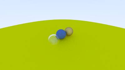
Image 20: A distant view

And we can change field of view:

    cam.vfov     = 20;

Listing 84: [main.cc] Change field of view

to get:

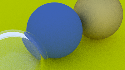
Image 21: Zooming in

   

Defocus Blur

Now our final feature: defocus blur. Note, photographers call this depth of field, so be sure to only use the term defocus blur among your raytracing friends.

The reason we have defocus blur in real cameras is because they need a big hole (rather than just a pinhole) through which to gather light. A large hole would defocus everything, but if we stick a lens in front of the film/sensor, there will be a certain distance at which everything is in focus. Objects placed at that distance will appear in focus and will linearly appear blurrier the further they are from that distance. You can think of a lens this way: all light rays coming from a specific point at the focus distance — and that hit the lens — will be bent back to a single point on the image sensor.

We call the distance between the camera center and the plane where everything is in perfect focus the focus distance. Be aware that the focus distance is not usually the same as the focal length — the focal length is the distance between the camera center and the image plane. For our model, however, these two will have the same value, as we will put our pixel grid right on the focus plane, which is focus distance away from the camera center.

In a physical camera, the focus distance is controlled by the distance between the lens and the film/sensor. That is why you see the lens move relative to the camera when you change what is in focus (that may happen in your phone camera too, but the sensor moves). The “aperture” is a hole to control how big the lens is effectively. For a real camera, if you need more light you make the aperture bigger, and will get more blur for objects away from the focus distance. For our virtual camera, we can have a perfect sensor and never need more light, so we only use an aperture when we want defocus blur.

   

A Thin Lens Approximation

A real camera has a complicated compound lens. For our code, we could simulate the order: sensor, then lens, then aperture. Then we could figure out where to send the rays, and flip the image after it’s computed (the image is projected upside down on the film). Graphics people, however, usually use a thin lens approximation:

 

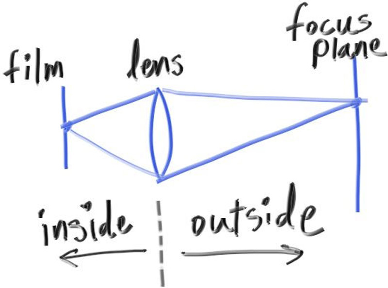
Figure 21: Camera lens model

We don’t need to simulate any of the inside of the camera — for the purposes of rendering an image outside the camera, that would be unnecessary complexity. Instead, I usually start rays from an infinitely thin circular “lens”, and send them toward the pixel of interest on the focus plane (focal_length away from the lens), where everything on that plane in the 3D world is in perfect focus.

In practice, we accomplish this by placing the viewport in this plane. Putting everything together:

1. The focus plane is orthogonal to the camera view direction.
2. The focus distance is the distance between the camera center and the focus plane.
3. The viewport lies on the focus plane, centered on the camera view direction vector.
4. The grid of pixel locations lies inside the viewport (located in the 3D world).
5. Random image sample locations are chosen from the region around the current pixel location.
6. The camera fires rays from random points on the lens through the current image sample location.

 

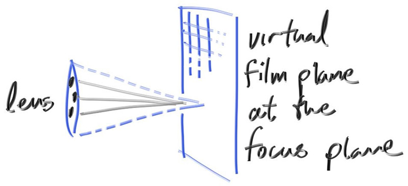
Figure 22: Camera focus plane

   

Generating Sample Rays

Without defocus blur, all scene rays originate from the camera center (or lookfrom). In order to accomplish defocus blur, we construct a disk centered at the camera center. The larger the radius, the greater the defocus blur. You can think of our original camera as having a defocus disk of radius zero (no blur at all), so all rays originated at the disk center (lookfrom).

So, how large should the defocus disk be? Since the size of this disk controls how much defocus blur we get, that should be a parameter of the camera class. We could just take the radius of the disk as a camera parameter, but the blur would vary depending on the projection distance. A slightly easier parameter is to specify the angle of the cone with apex at viewport center and base (defocus disk) at the camera center. This should give you more consistent results as you vary the focus distance for a given shot.

Since we’ll be choosing random points from the defocus disk, we’ll need a function to do that: random_in_unit_disk(). This function works using the same kind of method we use in random_in_unit_sphere(), just for two dimensions.

 

...
 
inline vec3 unit_vector(const vec3& u) {
    return v / v.length();
}
 
inline vec3 random_in_unit_disk() {
    while (true) {
        auto p = vec3(random_double(-1,1), random_double(-1,1), 0);
        if (p.length_squared() < 1)
            return p;
    }
}
...

Listing 85: [vec3.h] Generate random point inside unit disk

Now let’s update the camera to originate rays from the defocus disk:

 

class camera {
  public:
    double aspect_ratio      = 1.0;  // Ratio of image width over height
    int    image_width       = 100;  // Rendered image width in pixel count
    int    samples_per_pixel = 10;   // Count of random samples for each pixel
    int    max_depth         = 10;   // Maximum number of ray bounces into scene
 
    double vfov     = 90;              // Vertical view angle (field of view)
    point3 lookfrom = point3(0,0,0);   // Point camera is looking from
    point3 lookat   = point3(0,0,-1);  // Point camera is looking at
    vec3   vup      = vec3(0,1,0);     // Camera-relative "up" direction
 
    double defocus_angle = 0;  // Variation angle of rays through each pixel
    double focus_dist = 10;    // Distance from camera lookfrom point to plane of perfect focus
    ...
 
  private:
    int    image_height;         // Rendered image height
    double pixel_samples_scale;  // Color scale factor for a sum of pixel samples
    point3 center;               // Camera center
    point3 pixel00_loc;          // Location of pixel 0, 0
    vec3   pixel_delta_u;        // Offset to pixel to the right
    vec3   pixel_delta_v;        // Offset to pixel below
    vec3   u, v, w;              // Camera frame basis vectors    vec3   defocus_disk_u;       // Defocus disk horizontal radius
    vec3   defocus_disk_v;       // Defocus disk vertical radius
    void initialize() {
        image_height = int(image_width / aspect_ratio);
        image_height = (image_height < 1) ? 1 : image_height;
 
        pixel_samples_scale = 1.0 / samples_per_pixel;
 
        center = lookfrom;
 
        // Determine viewport dimensions.        auto focal_length = (lookfrom - lookat).length();        auto theta = degrees_to_radians(vfov);
        auto h = std::tan(theta/2);        auto viewport_height = 2 * h * focus_dist;        auto viewport_width = viewport_height * (double(image_width)/image_height);
 
        // Calculate the u,v,w unit basis vectors for the camera coordinate frame.
        w = unit_vector(lookfrom - lookat);
        u = unit_vector(cross(vup, w));
        v = cross(w, u);
 
        // Calculate the vectors across the horizontal and down the vertical viewport edges.
        vec3 viewport_u = viewport_width * u;    // Vector across viewport horizontal edge
        vec3 viewport_v = viewport_height * -v;  // Vector down viewport vertical edge
 
        // Calculate the horizontal and vertical delta vectors to the next pixel.
        pixel_delta_u = viewport_u / image_width;
        pixel_delta_v = viewport_v / image_height;
 
        // Calculate the location of the upper left pixel.        auto viewport_upper_left = center - (focus_dist * w) - viewport_u/2 - viewport_v/2;        pixel00_loc = viewport_upper_left + 0.5 * (pixel_delta_u + pixel_delta_v);
 
        // Calculate the camera defocus disk basis vectors.
        auto defocus_radius = focus_dist * std::tan(degrees_to_radians(defocus_angle / 2));
        defocus_disk_u = u * defocus_radius;
        defocus_disk_v = v * defocus_radius;    }
 
    ray get_ray(int i, int j) const {        // Construct a camera ray originating from the defocus disk and directed at a randomly
        // sampled point around the pixel location i, j.
        auto offset = sample_square();
        auto pixel_sample = pixel00_loc
                          + ((i + offset.x()) * pixel_delta_u)
                          + ((j + offset.y()) * pixel_delta_v);
 
        auto ray_origin = (defocus_angle <= 0) ? center : defocus_disk_sample();        auto ray_direction = pixel_sample - ray_origin;
 
        return ray(ray_origin, ray_direction);
    }
 
    vec3 sample_square() const {
        ...
    }
 
    point3 defocus_disk_sample() const {
        // Returns a random point in the camera defocus disk.
        auto p = random_in_unit_disk();
        return center + (p[0] * defocus_disk_u) + (p[1] * defocus_disk_v);
    }
    color ray_color(const ray& r, int depth, const hittable& world) const {
        ...
    }
};

Listing 86: [camera.h] Camera with adjustable depth-of-field

Using a large aperture:

int main() {
    ...
 
    camera cam;
 
    cam.aspect_ratio      = 16.0 / 9.0;
    cam.image_width       = 400;
    cam.samples_per_pixel = 100;
    cam.max_depth         = 50;
 
    cam.vfov     = 20;
    cam.lookfrom = point3(-2,2,1);
    cam.lookat   = point3(0,0,-1);
    cam.vup      = vec3(0,1,0);
 
    cam.defocus_angle = 10.0;
    cam.focus_dist    = 3.4;
    cam.render(world);
}

Listing 87: [main.cc] Scene camera with depth-of-field

We get:

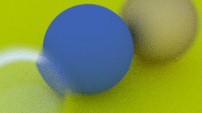
Image 22: Spheres with depth-of-field

   

Where Next?

   

A Final Render

Let’s make the image on the cover of this book — lots of random spheres.

 

int main() {
    hittable_list world;
 
    auto ground_material = make_shared<lambertian>(color(0.5, 0.5, 0.5));
    world.add(make_shared<sphere>(point3(0,-1000,0), 1000, ground_material));
 
    for (int a = -11; a < 11; a++) {
        for (int b = -11; b < 11; b++) {
            auto choose_mat = random_double();
            point3 center(a + 0.9*random_double(), 0.2, b + 0.9*random_double());
 
            if ((center - point3(4, 0.2, 0)).length() > 0.9) {
                shared_ptr<material> sphere_material;
 
                if (choose_mat < 0.8) {
                    // diffuse
                    auto albedo = color::random() * color::random();
                    sphere_material = make_shared<lambertian>(albedo);
                    world.add(make_shared<sphere>(center, 0.2, sphere_material));
                } else if (choose_mat < 0.95) {
                    // metal
                    auto albedo = color::random(0.5, 1);
                    auto fuzz = random_double(0, 0.5);
                    sphere_material = make_shared<metal>(albedo, fuzz);
                    world.add(make_shared<sphere>(center, 0.2, sphere_material));
                } else {
                    // glass
                    sphere_material = make_shared<dielectric>(1.5);
                    world.add(make_shared<sphere>(center, 0.2, sphere_material));
                }
            }
        }
    }
 
    auto material1 = make_shared<dielectric>(1.5);
    world.add(make_shared<sphere>(point3(0, 1, 0), 1.0, material1));
 
    auto material2 = make_shared<lambertian>(color(0.4, 0.2, 0.1));
    world.add(make_shared<sphere>(point3(-4, 1, 0), 1.0, material2));
 
    auto material3 = make_shared<metal>(color(0.7, 0.6, 0.5), 0.0);
    world.add(make_shared<sphere>(point3(4, 1, 0), 1.0, material3));
    camera cam;
 
    cam.aspect_ratio      = 16.0 / 9.0;
    cam.image_width       = 1200;
    cam.samples_per_pixel = 500;
    cam.max_depth         = 50;
 
    cam.vfov     = 20;
    cam.lookfrom = point3(13,2,3);
    cam.lookat   = point3(0,0,0);
    cam.vup      = vec3(0,1,0);
 
    cam.defocus_angle = 0.6;
    cam.focus_dist    = 10.0;
    cam.render(world);
}

Listing 88: [main.cc] Final scene

(Note that the code above differs slightly from the project sample code: the samples_per_pixel is set to 500 above for a high-quality image that will take quite a while to render. The project source code uses a value of 10 in the interest of reasonable run times while developing and validating.)

This gives:

Image 23: Final scene

An interesting thing you might note is the glass balls don’t really have shadows which makes them look like they are floating. This is not a bug — you don’t see glass balls much in real life, where they also look a bit strange, and indeed seem to float on cloudy days. A point on the big sphere under a glass ball still has lots of light hitting it because the sky is re-ordered rather than blocked.

   

Next Steps

You now have a cool ray tracer! What next?

   

Book 2: Ray Tracing: The Next Week

The second book in this series builds on the ray tracer you’ve developed here. This includes new features such as:

• Motion blur — Realistically render moving objects.
• Bounding volume hierarchies — speeding up the rendering of complex scenes.
• Texture maps — placing images on objects.
• Perlin noise — a random noise generator very useful for many techniques.
• Quadrilaterals — something to render besides spheres! Also, the foundation to implement disks, triangles, rings or just about any other 2D primitive.
• Lights — add sources of light to your scene.
• Transforms — useful for placing and rotating objects.
• Volumetric rendering — render smoke, clouds and other gaseous volumes.

   

Book 3: Ray Tracing: The Rest of Your Life

This book expands again on the content from the second book. A lot of this book is about improving both the rendered image quality and the renderer performance, and focuses on generating the right rays and accumulating them appropriately.

This book is for the reader seriously interested in writing professional-level ray tracers, and/or interested in the foundation to implement advanced effects like subsurface scattering or nested dielectrics.

   

Other Directions

There are so many additional directions you can take from here, including techniques we haven’t (yet?) covered in this series. These include:

Triangles — Most cool models are in triangle form. The model I/O is the worst and almost everybody tries to get somebody else’s code to do this. This also includes efficiently handling large meshes of triangles, which present their own challenges.

Parallelism — Run $N$ copies of your code on $N$ cores with different random seeds. Average the $N$ runs. This averaging can also be done hierarchically where $N/2$ pairs can be averaged to get $N/4$ images, and pairs of those can be averaged. That method of parallelism should extend well into the thousands of cores with very little coding.

Shadow Rays — When firing rays at light sources, you can determine exactly how a particular point is shadowed. With this, you can render crisp or soft shadows, adding another degreee of realism to your scenes.

Have fun, and please send me your cool images!

   

Acknowledgments

Original Manuscript Help

• Dave Hart
• Jean Buckley

Corrections and Improvements

• Aaryaman Vasishta
• Andrew Kensler
• Antonio Gamiz
• Apoorva Joshi
• Aras Pranckevičius
• Arman Uguray
• Becker
• Ben Kerl
• Benjamin Summerton
• Bennett Hardwick
• Benny Tsang
• Dan Drummond
• David Chambers
• David Hart
• Dimitry Ishenko
• Dmitry Lomov
• Eric Haines
• Fabio Sancinetti
• Filipe Scur
• Frank He
• Gareth Martin
• Gerrit Wessendorf
• Grue Debry
• Gustaf Waldemarson
• Ingo Wald
• Jason Stone
• JC-ProgJava
• Jean Buckley
• Jeff Smith
• Joey Cho
• John Kilpatrick
• Kaan Eraslan
• Lorenzo Mancini
• Manas Kale
• Marcus Ottosson
• Mark Craig
• Markus Boos
• Matthew Heimlich
• Nakata Daisuke
• Nate Rupsis
• Paul Melis
• Phil Cristensen
• LollipopFt
• Ronald Wotzlaw
• Shaun P. Lee
• Shota Kawajiri
• Tatsuya Ogawa
• Thiago Ize
• Thien Tran
• Vahan Sosoyan
• WANG Lei
• Yann Herklotz
• ZeHao Chen

Special Thanks

Thanks to the team at Limnu for help on the figures.

These books are entirely written in Morgan McGuire’s fantastic and free Markdeep library. To see what this looks like, view the page source from your browser.

Thanks to Helen Hu for graciously donating her https://github.com/RayTracing/ GitHub organization to this project.

   

Citing This Book

Consistent citations make it easier to identify the source, location and versions of this work. If you are citing this book, we ask that you try to use one of the following forms if possible.

   

Basic Data

• Title (series): “Ray Tracing in One Weekend Series”
• Title (book): “Ray Tracing in One Weekend”
• Author: Peter Shirley, Trevor David Black, Steve Hollasch
• Version/Edition: v4.0.1
• Date: 2024-08-30
• URL (series): https://raytracing.github.io
• URL (book): https://raytracing.github.io/books/raytracinginoneweekend.html

   

Snippets

   

Markdown

[_Ray Tracing in One Weekend_](https://raytracing.github.io/books/RayTracingInOneWeekend.html)

   

HTML

<a href="https://raytracing.github.io/books/RayTracingInOneWeekend.html">
    <cite>Ray Tracing in One Weekend</cite>
</a>

   

LaTeX and BibTex

~\cite{Shirley2024RTW1}
 
@misc{Shirley2024RTW1,
   title = {Ray Tracing in One Weekend},
   author = {Peter Shirley, Trevor David Black, Steve Hollasch},
   year = {2024},
   month = {August},
   note = {\small \texttt{https://raytracing.github.io/books/RayTracingInOneWeekend.html}},
   url = {https://raytracing.github.io/books/RayTracingInOneWeekend.html}
}

   

BibLaTeX

\usepackage{biblatex}
 
~\cite{Shirley2024RTW1}
 
@online{Shirley2024RTW1,
   title = {Ray Tracing in One Weekend},
   author = {Peter Shirley, Trevor David Black, Steve Hollasch},
   year = {2024},
   month = {August},
   url = {https://raytracing.github.io/books/RayTracingInOneWeekend.html}
}

   

IEEE

“Ray Tracing in One Weekend.” raytracing.github.io/books/RayTracingInOneWeekend.html
(accessed MMM. DD, YYYY)

   

MLA:

Ray Tracing in One Weekend. raytracing.github.io/books/RayTracingInOneWeekend.html
Accessed DD MMM. YYYY.