The Gram-Schmidt process (or procedure) is a sequence of operations that allow us to transform a set of linearly independent vectors into a set of orthonormal vectors that span the same space spanned by the original set.
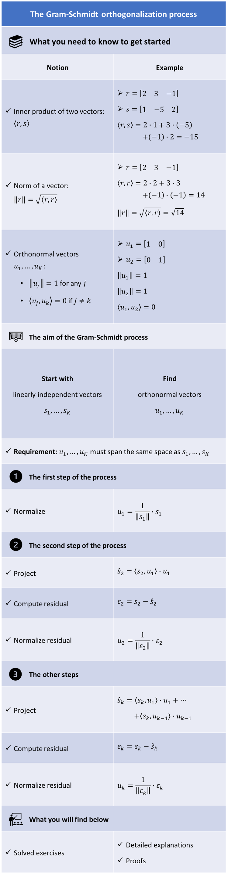
Table of contents
Preliminaries
Let us review some notions that are essential to understand the Gram-Schmidt process.
Remember that two vectors and
are said to be orthogonal if and only if their inner product is equal to zero, that is,
Given an inner product, we can define the norm (length) of a vector as follows:
A set of vectors is called orthonormal if and only if its elements have unit norm and are orthogonal to each other. In other words, a set of vectors
is orthonormal if and only if
We have proved that the vectors of an orthonormal set are linearly independent.
When a basis for a vector space is also an orthonormal set, it is called an orthonormal basis.
Projections on orthonormal sets
In the Gram-Schmidt process, we repeatedly use the next proposition, which shows that every vector can be decomposed into two parts: 1) its projection on an orthonormal set and 2) a residual that is orthogonal to the given orthonormal set.
Proposition Let be a vector space equipped with an inner product
. Let
be an orthonormal set. For any
, we have
where
is orthogonal to
for any
Proof
The termis called the linear projection of
on the orthonormal set
, while the term
is called the residual of the linear projection.
Normalization
Another perhaps obvious fact that we are going to repeatedly use in the Gram-Schmidt process is that, if we take any non-zero vector and we divide it by its norm, then the result of the division is a new vector that has unit norm.
In other words, if then, by the definiteness property of the norm, we have that
As a consequence, we can defineand, by the positivity and absolute homogeneity of the norm, we have
Overview of the procedure
Now that we know how to normalize a vector and how to decompose it into a projection on an orthonormal set and a residual, we are ready to explain the Gram-Schmidt procedure.
We are going to provide an overview of the process, after which we will express it formally as a proposition and we will discuss all the technical details in the proof of the proposition.
Here is the overview.
We are given a set of linearly independent vectors .
To start the process, we normalize the first vector, that is, we define
In the second step, we project on
:
where
is the residual of the projection.
Then, we normalize the residual:
We will later prove that (so that the normalization can be performed) because the starting vectors are linearly independent.
The two vectors and
thus obtained are orthonormal.
In the third step, we project on
and
:
and we compute the residual of the projection
.
We then normalize it:
We proceed in this manner until we obtain the last normalized residual .
At the end of the process, the vectors form an orthonormal set because:
- they are the result of a normalization, and as a consequence they have unit norm;
- each
is obtained from a residual that has the property of being orthogonal to
To complete this overview, let us remember that the linear span of is the set of all vectors that can be written as linear combinations of
; it is denoted by
and it is a linear space.
Since the vectors are linearly independent combinations of
, any vector that can be written as a linear combination of
can also be written as a linear combination of
. Therefore, the spans of the two sets of vectors coincide:
Formal statement
We formalize here the Gram-Schmidt process as a proposition, whose proof contains all the technical details of the procedure.
Proposition Let be a vector space equipped with an inner product
. Let
be linearly independent vectors. Then, there exists a set of orthonormal vectors
such that
for any
.
Proof
The proof is by induction: first we prove that the proposition is true for , and then we prove that it is true for a generic
if it holds for
. When
, the vector
has unit norm and it constitutes by itself an orthonormal set: there are no other vectors, so the orthogonality condition is trivially satisfied. The set
is the set of all scalar multiples of
, which are also scalar multiples of
(and vice versa). Therefore,
Now, suppose that the proposition is true for
. Then, we can project
on
:
where the residual
is orthogonal to
. Suppose that
. Then,
Since, by assumption,
for any
, we have that
for any
, where
are scalars. Therefore,
In other words, the assumption that
leads to the conclusion that
is a linear combination of
. But this is impossible because one of the assumptions of the proposition is that
are linearly independent. As a consequence, it must be that
. We can therefore normalize the residual and define the vector
which has unit norm. We already know that
is orthogonal to
. This implies that also
is orthogonal to
. Thus,
is an orthonormal set. Now, take any vector
that can be written as
where
are scalars. Since, by assumption,
![[eq57]](https://www.statlect.com/images/Gram-Schmidt-process__107.png) we have that equation (2) can also be written as
we have that equation (2) can also be written as![[eq58]](https://www.statlect.com/images/Gram-Schmidt-process__108.png) where
where are scalars, and: in step
we have used equation (1); in step
we have used the definition of
. Thus, we have proved that every vector that can be written as a linear combination of
can also be written as a linear combination of
. Assumption (3) allows us to prove the converse in a completely analogous manner:
![[eq62]](https://www.statlect.com/images/Gram-Schmidt-process__115.png) In other words, every linear combination of
In other words, every linear combination of is also a linear combination of
. This proves that
and concludes the proof.
Every inner product space has an orthonormal basis
The following proposition presents an important consequence of the Gram-Schmidt process.
Proposition Let be a vector space equipped with an inner product
. If
has finite dimension
, then there exists an orthonormal basis
for
.
Proof
Solved exercises
Below you can find some exercises with explained solutions.
Exercise 1
Consider the space of all
vectors having real entries and the inner product
where
and
is the transpose of
.
Define the vector
Normalize .
Solution
The norm of is
Therefore, the normalization of
is
![[eq77]](https://www.statlect.com/images/Gram-Schmidt-process__146.png)
Exercise 2
Consider the space of all
vectors having real entries and the inner product
where
.
Consider the two linearly independent vectors
Transform them into an orthonormal set by using the Gram-Schmidt process.
Solution
The norm of is
Therefore, the first orthonormal vector is
The inner product of
and
is
![[eq82]](https://www.statlect.com/images/Gram-Schmidt-process__157.png) The projection of
The projection of on
is
![[eq83]](https://www.statlect.com/images/Gram-Schmidt-process__160.png) The residual of the projection is
The residual of the projection isThe norm of the residual is
and the normalized residual is
Thus, the orthonormal set we were looking for is
![[eq87]](https://www.statlect.com/images/Gram-Schmidt-process__164.png)
How to cite
Please cite as:
Taboga, Marco (2021). “Gram-Schmidt process”, Lectures on matrix algebra. https://www.statlect.com/matrix-algebra/Gram-Schmidt-process.