Adversarial attacks with FGSM (Fast Gradient Sign Method) - PyImageSearch

In this tutorial, you will learn how to perform adversarial attacks using the Fast Gradient Sign Method (FGSM). We will implement FGSM using Keras and TensorFlow.

A dataset of images and their labels is critical for understanding adversarial attacksusing FGSM. It enables us to see how these attacks can manipulate the input to the model, leading to incorrect predictions.

Roboflow has free tools for each stage of the computer vision pipeline that will streamline your workflows and supercharge your productivity.

Sign up or Log in to your Roboflow account to access state of the art dataset libaries and revolutionize your computer vision pipeline.

You can start by choosing your own datasets or using our PyimageSearch’s assorted library of useful datasets.

Bring data in any of 40+ formats to Roboflow, train using any state-of-the-art model architectures, deploy across multiple platforms (API, NVIDIA, browser, iOS, etc), and connect to applications or 3rd party tools.

Previously, we learned how to implement two forms of adversarial image attacks:

1. Untargeted adversarial attacks, where we cannot control the output label of the adversarial image.
2. Targeted adversarial attacks, where we can control the output label of the image.

Today we’re going to look at another untargeted adversarial image generation method called the Fast Gradient Sign Method (FGSM). As you’ll see, this method is super easy to implement.

Then, in the next two weeks, you’ll learn how to defend against adversarial attacks by updating your training procedure to utilize FGSM, thereby improving the accuracy and robustness of your model.

To learn how to perform adversarial attacks with the Fast Gradient Sign Method, just keep reading.

Looking for the source code to this post?

Jump Right To The Downloads Section

In the first part of this tutorial, you’ll learn about the Fast Gradient Sign Method and its use for adversarial image generation.

From there, we’ll configure our development environment and review our project directory structure.

We’ll then implement three Python scripts:

1. The first one will contain

SimpleCNN

SimpleCNN, our implementation of a basic CNN that we’ll train on the MNIST dataset. 2. Our second Python script will contain our implementation of the FGSM for adversarial image generation. 3. Finally, our third script will train our CNN on MNIST and then demonstrate how to use FGSM to fool our trained CNN into making incorrect predictions.

If you haven’t yet, I recommend that you read my previous two tutorials on adversarial image generation:

1. Adversarial images and attacks with Keras and TensorFlow
2. Targeted adversarial attacks with Keras and TensorFlow

These two guides are considered required reading as I’ll be assuming you already know the basics of adversarial image generation. If you haven’t read those tutorials yet, I suggest you stop now and read them first.

The Fast Gradient Sign Method (FGSM)

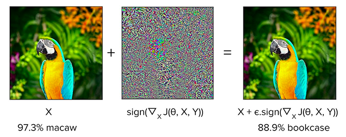
Figure 1: The Fast Gradient Sign Method (FGSM) for adversarial image generation (image source).

The Fast Gradient Sign Method (FGSM) is a simple yet effective method to generate adversarial images. First introduced by Goodfellow et al. in their paper, Explaining and Harnessing Adversarial Examples, FGSM works by:

1. Taking an input image
2. Making predictions on the image using a trained CNN
3. Computing the loss of the prediction based on the true class label
4. Calculating the gradients of the loss with respect to the input image
5. Computing the sign of the gradient
6. Using the signed gradient to construct the output adversarial image

This process may sound complicated, but as you’ll see, we’ll be able to implement the entire FGSM function in under 30 lines of code (including comments).

How does the Fast Gradient Sign Method work?

The FGSM exploits the gradients of a neural network to build an adversarial image, similar to what we’ve done in the untargeted adversarial attack and targeted adversarial attack tutorials.

Essentially, FGSM computes the gradients of a loss function (e.g., mean-squared error or categorical cross-entropy) with respect to the input image and then uses the sign of the gradients to create a new image (i.e., the adversarial image) that maximizes the loss.

The result is an output image that, according to the human eye, looks identical to the original, but makes the neural network make an incorrect prediction!

Quoting the TensorFlow documentation on FGSM, we can express the Fast Gradient Sign Method using the following equation:

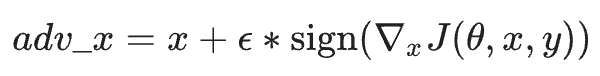
Figure 2: The Fast Gradient Sign Method expressed mathematically (image source).

where:

If you’re struggling to follow the math surrounding FGSM, don’t worry, it will be much easier to understand once we start looking at some code later in this guide.

Configuring your development environment

This tutorial on adversarial images with FGSM utilizes Keras and TensorFlow. If you intend to follow this tutorial, I suggest you take the time to configure your deep learning development environment.

You can utilize either of these two guides to install TensorFlow and Keras on your system:

• How to install TensorFlow 2.0 on Ubuntu
• How to install TensorFlow 2.0 on macOS

Either tutorial will help configure your system with all the necessary software for this blog post in a convenient Python virtual environment.

Having problems configuring your development environment?

Figure 3: Having trouble configuring your dev environment? Want access to pre-configured Jupyter Notebooks running on Google Colab? Be sure to join PyImageSearch Plus — you’ll be up and running with this tutorial in a matter of minutes.

All that said, are you:

• Short on time?
• Learning on your employer’s administratively locked system?
• Wanting to skip the hassle of fighting with the command line, package managers, and virtual environments?
• Ready to run the code right now on your Windows, macOS, or Linux systems?

Then join PyImageSearch Plus today!

Gain access to Jupyter Notebooks for this tutorial and other PyImageSearch guides that are pre-configured to run on Google Colab’s ecosystem right in your web browser! No installation required.

And best of all, these Jupyter Notebooks will run on Windows, macOS, and Linux!

Project structure

Let’s get started by reviewing our project directory structure. Be sure to access the “Downloads” section of this tutorial to retrieve the source code:

Adversarial attacks with FGSM (Fast Gradient Sign Method)

$ tree . —dirsfirst . ├── pyimagesearch │ ├── __init__.py │ ├── fgsm.py │ └── simplecnn.py └── fgsm_adversarial.py 1 directory, 4 files

$ tree . --dirsfirst
.
├── pyimagesearch
│   ├── __init__.py
│   ├── fgsm.py
│   └── simplecnn.py
└── fgsm_adversarial.py

1 directory, 4 files

Inside the

pyimagesearch

pyimagesearch module, we have two Python scripts we’ll be implementing:

1. simplecnn.py

simplecnn.py: A basic CNN architecture 2. fgsm.py

fgsm.py: Our implementation of the Fast Gradient Sign Method adversarial attack

The

fgsm_adversarial.py

fgsm_adversarial.py file is our driver script. It will:

1. Instantiate an instance of

SimpleCNN

SimpleCNN 2. Train it on the MNIST dataset 3. Demonstrate how to apply the FGSM adversarial attack to the trained model

Creating a simple CNN architecture for adversarial training

Before we can perform an adversarial attack, we first need to implement our CNN architecture.

Once our architecture is implemented, we’ll train it on the MNIST dataset, evaluate it, generate a set of adversarial images using the FGSM, and re-evaluate it, thereby demonstrating the impact adversarial images have on accuracy.

In next week and the following week’s tutorials, you’ll learn training techniques that you can use to defend against these adversarial attacks.

But it all starts with implementing the CNN architecture — open the

simplecnn.py

simplecnn.py in the

pyimagesearch

pyimagesearch module of our project directory structure and let’s get to work:

Adversarial attacks with FGSM (Fast Gradient Sign Method)

# import the necessary packages

from tensorflow.keras.models import Sequential

from tensorflow.keras.layers import BatchNormalization

from tensorflow.keras.layers import Conv2D

from tensorflow.keras.layers import Activation

from tensorflow.keras.layers import Flatten

from tensorflow.keras.layers import Dropout

from tensorflow.keras.layers import Dense

# import the necessary packages from tensorflow.keras.models import Sequential from tensorflow.keras.layers import BatchNormalization from tensorflow.keras.layers import Conv2D from tensorflow.keras.layers import Activation from tensorflow.keras.layers import Flatten from tensorflow.keras.layers import Dropout from tensorflow.keras.layers import Dense

# import the necessary packages
from tensorflow.keras.models import Sequential
from tensorflow.keras.layers import BatchNormalization
from tensorflow.keras.layers import Conv2D
from tensorflow.keras.layers import Activation
from tensorflow.keras.layers import Flatten
from tensorflow.keras.layers import Dropout
from tensorflow.keras.layers import Dense

We start on Lines 2-8, importing our required Keras/TensorFlow classes. These are all fairly standard imports when training a CNN.

If you’re new to Keras and TensorFlow, I suggest you read my introductory Keras tutorial along with my book, Deep Learning for Computer Vision with Python, which covers deep learning in detail.

With our imports taken care of, we can define our CNN architecture:

Adversarial attacks with FGSM (Fast Gradient Sign Method)

def build(width, height, depth, classes):

# initialize the model along with the input shape

inputShape = (height, width, depth)

# first CONV ⇒ RELU ⇒ BN layer set

model.add(Conv2D(32, (3, 3), strides=(2, 2), padding=“same”,

model.add(Activation(“relu”))

model.add(BatchNormalization(axis=chanDim))

# second CONV ⇒ RELU ⇒ BN layer set

model.add(Conv2D(64, (3, 3), strides=(2, 2), padding=“same”))

model.add(Activation(“relu”))

model.add(BatchNormalization(axis=chanDim))

# first (and only) set of FC ⇒ RELU layers

model.add(Activation(“relu”))

model.add(BatchNormalization())

model.add(Dense(classes))

model.add(Activation(“softmax”))

# return the constructed network architecture

class SimpleCNN: @staticmethod def build(width, height, depth, classes): # initialize the model along with the input shape model = Sequential() inputShape = (height, width, depth) chanDim = -1 # first CONV ⇒ RELU ⇒ BN layer set model.add(Conv2D(32, (3, 3), strides=(2, 2), padding=“same”, input_shape=inputShape)) model.add(Activation(“relu”)) model.add(BatchNormalization(axis=chanDim)) # second CONV ⇒ RELU ⇒ BN layer set model.add(Conv2D(64, (3, 3), strides=(2, 2), padding=“same”)) model.add(Activation(“relu”)) model.add(BatchNormalization(axis=chanDim)) # first (and only) set of FC ⇒ RELU layers model.add(Flatten()) model.add(Dense(128)) model.add(Activation(“relu”)) model.add(BatchNormalization()) model.add(Dropout(0.5)) # softmax classifier model.add(Dense(classes)) model.add(Activation(“softmax”)) # return the constructed network architecture return model

class SimpleCNN:
	@staticmethod
	def build(width, height, depth, classes):
		# initialize the model along with the input shape
		model = Sequential()
		inputShape = (height, width, depth)
		chanDim = -1

		# first CONV => RELU => BN layer set
		model.add(Conv2D(32, (3, 3), strides=(2, 2), padding="same",
			input_shape=inputShape))
		model.add(Activation("relu"))
		model.add(BatchNormalization(axis=chanDim))

		# second CONV => RELU => BN layer set
		model.add(Conv2D(64, (3, 3), strides=(2, 2), padding="same"))
		model.add(Activation("relu"))
		model.add(BatchNormalization(axis=chanDim))

		# first (and only) set of FC => RELU layers
		model.add(Flatten())
		model.add(Dense(128))
		model.add(Activation("relu"))
		model.add(BatchNormalization())
		model.add(Dropout(0.5))

		# softmax classifier
		model.add(Dense(classes))
		model.add(Activation("softmax"))

		# return the constructed network architecture
		return model

The

build

build method of our

SimpleCNN

SimpleCNN class accepts four parameters:

1. width

width: Width of the input images in our dataset 2. height

height: Height of the input images in our dataset 3. channels

channels: Number of channels in the images 4. classes

classes: Total number of unique classes in the dataset

From there, we define a

Sequential

Sequential network consisting of:

1. **A first set of

CONV ⇒ RELU ⇒ BN

CONV => RELU => BN layers.** The

CONV

CONV layer learns a total of 32 3×3 filters with 2×2 strided convolution to reduce volume size. 2. **A second set of

CONV ⇒ RELU ⇒ BN

CONV => RELU => BN layers.** Same as above, but this time the

CONV

CONV layer learns 64 filters. 3. A set of dense/fully-connected layers. The output of which is our softmax classifier used for returning probabilities for each class label.

Now that our architecture has been implemented, we can move on to the Fast Gradient Sign Method.

Implementing the Fast Gradient Sign Method with Keras and TensorFlow

The adversarial attack method we will implement is called the Fast Gradient Sign Method (FGSM). It’s called this method because:

1. It’s fast (it’s in the name)
2. We construct the image adversary by calculating the gradients of the loss, computing the sign of the gradient, and then using the sign to build the image adversary

Let’s implement the FGSM now. Open the

fgsm.py

fgsm.py file in your project directory structure and insert the following code:

Adversarial attacks with FGSM (Fast Gradient Sign Method)

# import the necessary packages

from tensorflow.keras.losses import MSE

def generate_image_adversary(model, image, label, eps=2 / 255.0):

image = tf.cast(image, tf.float32)

# import the necessary packages from tensorflow.keras.losses import MSE import tensorflow as tf def generate_image_adversary(model, image, label, eps=2 / 255.0): # cast the image image = tf.cast(image, tf.float32)

# import the necessary packages
from tensorflow.keras.losses import MSE
import tensorflow as tf

def generate_image_adversary(model, image, label, eps=2 / 255.0):
	# cast the image
	image = tf.cast(image, tf.float32)

Lines 2 and 3 import our required Python packages. We’ll be using the mean-squared error (

MSE

MSE) loss function for computing our adversarial attack, but you could also use any other appropriate loss function for the task, including categorical cross-entropy, binary cross-entropy, etc.

Line 5 starts the definition of our FGSM attack,

generate_image_adversary

generate_image_adversary. This function accepts four parameters:

1. The

model

model that we are trying to fool 2. The input

image

image that we want to misclassify 3. The ground-truth class

label

label of the input image 4. A small

eps

eps value that weights the gradient update — a small-ish value should be used here such that the gradient update is large enough to cause the input image to be misclassified but not so large that the human eye can tell the image has been manipulated

Let’s start implementing the FGSM attack now:

Adversarial attacks with FGSM (Fast Gradient Sign Method)

with tf.GradientTape() as tape:

# explicitly indicate that our image should be tacked for

# use our model to make predictions on the input image and

# record our gradients with tf.GradientTape() as tape: # explicitly indicate that our image should be tacked for # gradient updates tape.watch(image) # use our model to make predictions on the input image and # then compute the loss pred = model(image) loss = MSE(label, pred)

	# record our gradients
	with tf.GradientTape() as tape:
		# explicitly indicate that our image should be tacked for
		# gradient updates
		tape.watch(image)

		# use our model to make predictions on the input image and
		# then compute the loss
		pred = model(image)
		loss = MSE(label, pred)

Line 10 instructs TensorFlow to record our gradients, while Line 13 explicitly tells TensorFlow that we want to track the gradient updates on our input

image

image.

From there, we use our

model

model to make predictions on the image and then compute our loss using mean-squared error (again, you can substitute another loss function here for your task, but MSE is a fairly standard choice).

Next, let’s implement the “signed gradient” portion of the FGSM attack:

Adversarial attacks with FGSM (Fast Gradient Sign Method)

# calculate the gradients of loss with respect to the image, then

# compute the sign of the gradient

gradient = tape.gradient(loss, image)

signedGrad = tf.sign(gradient)

# construct the image adversary

adversary = (image + (signedGrad * eps)).numpy()

# return the image adversary to the calling function

# calculate the gradients of loss with respect to the image, then # compute the sign of the gradient gradient = tape.gradient(loss, image) signedGrad = tf.sign(gradient) # construct the image adversary adversary = (image + (signedGrad * eps)).numpy() # return the image adversary to the calling function return adversary

	# calculate the gradients of loss with respect to the image, then
	# compute the sign of the gradient
	gradient = tape.gradient(loss, image)
	signedGrad = tf.sign(gradient)

	# construct the image adversary
	adversary = (image + (signedGrad * eps)).numpy()

	# return the image adversary to the calling function
	return adversary

Line 22 computes the gradients of the loss with respect to the image.

We then take the sign of the gradient on Line 23 (hence the term, Fast Gradient Sign Method). The output of this line of code is a vector filled with three values — either

1

1 (positive),

0

0, or

-1

-1 (negative).

Using this information, Line 26 creates our image adversary by:

1. Taking the signed gradient and multiplying it by a small epsilon factor. The goal here is to make our gradient update large enough to misclassify the input image but not so large that the human eye can tell the image has been tampered.
2. We then add this small delta value to our image, which ever so slightly changes the pixel intensity values in the image.

These pixel updates will be undetectable to the human eye, but according to our CNN, the image will appear vastly different**, resulting in misclassification.**

Creating our adversarial training script

With both our CNN architecture and FGSM implemented, we can move on to creating our training script.

Open the

fgsm_adversarial.py

fgsm_adversarial.py script in our directory structure, and we can get to work:

Adversarial attacks with FGSM (Fast Gradient Sign Method)

# import the necessary packages

from pyimagesearch.simplecnn import SimpleCNN

from pyimagesearch.fgsm import generate_image_adversary

from tensorflow.keras.optimizers import Adam

from tensorflow.keras.utils import to_categorical

from tensorflow.keras.datasets import mnist

# import the necessary packages from pyimagesearch.simplecnn import SimpleCNN from pyimagesearch.fgsm import generate_image_adversary from tensorflow.keras.optimizers import Adam from tensorflow.keras.utils import to_categorical from tensorflow.keras.datasets import mnist import numpy as np import cv2

# import the necessary packages
from pyimagesearch.simplecnn import SimpleCNN
from pyimagesearch.fgsm import generate_image_adversary
from tensorflow.keras.optimizers import Adam
from tensorflow.keras.utils import to_categorical
from tensorflow.keras.datasets import mnist
import numpy as np
import cv2

Lines 2-8 import our required Python packages. Our notable imports include

SimpleCNN

SimpleCNN (our basic CNN architecture we implemented earlier in this guide) and

generate_image_adversary

generate_image_adversary (our helper function to perform the FGSM attack).

We’ll be training our

SimpleCNN

SimpleCNN architecture on the

mnist

mnist dataset. The model will be trained with categorical cross-entropy loss and the

Adam

Adam optimizer.

With the imports taken care of, we can now load the MNIST dataset from disk:

Adversarial attacks with FGSM (Fast Gradient Sign Method)

# load MNIST dataset and scale the pixel values to the range [0, 1]

print(“[INFO] loading MNIST dataset…“)

(trainX, trainY), (testX, testY) = mnist.load_data()

# add a channel dimension to the images

trainX = np.expand_dims(trainX, axis=-1)

testX = np.expand_dims(testX, axis=-1)

# one-hot encode our labels

trainY = to_categorical(trainY, 10)

testY = to_categorical(testY, 10)

# load MNIST dataset and scale the pixel values to the range [0, 1] print(“[INFO] loading MNIST dataset…“) (trainX, trainY), (testX, testY) = mnist.load_data() trainX = trainX / 255.0 testX = testX / 255.0 # add a channel dimension to the images trainX = np.expand_dims(trainX, axis=-1) testX = np.expand_dims(testX, axis=-1) # one-hot encode our labels trainY = to_categorical(trainY, 10) testY = to_categorical(testY, 10)

# load MNIST dataset and scale the pixel values to the range [0, 1]
print("[INFO] loading MNIST dataset...")
(trainX, trainY), (testX, testY) = mnist.load_data()
trainX = trainX / 255.0
testX = testX / 255.0

# add a channel dimension to the images
trainX = np.expand_dims(trainX, axis=-1)
testX = np.expand_dims(testX, axis=-1)

# one-hot encode our labels
trainY = to_categorical(trainY, 10)
testY = to_categorical(testY, 10)

Line 12 loads the pre-split MNIST dataset from disk. We preprocess the MNIST dataset by:

1. Scaling the pixel intensities from the range [0, 255] to [0, 1]
2. Adding a batch dimension to the images
3. One-hot encoding the labels

From there, we can initialize our

SimpleCNN

SimpleCNN model:

Adversarial attacks with FGSM (Fast Gradient Sign Method)

# initialize our optimizer and model

print(“[INFO] compiling model…”)

model = SimpleCNN.build(width=28, height=28, depth=1, classes=10)

model.compile(loss=“categorical_crossentropy”, optimizer=opt,

# train the simple CNN on MNIST

print(“[INFO] training network…”)

model.fit(trainX, trainY,

validation_data=(testX, testY),

# make predictions on the testing set for the model trained on

(loss, acc) = model.evaluate(x=testX, y=testY, verbose=0)

print(“[INFO] loss: {:.4f}, acc: {:.4f}“.format(loss, acc))

# initialize our optimizer and model print(“[INFO] compiling model…”) opt = Adam(lr=1e-3) model = SimpleCNN.build(width=28, height=28, depth=1, classes=10) model.compile(loss=“categorical_crossentropy”, optimizer=opt, metrics=[“accuracy”]) # train the simple CNN on MNIST print(“[INFO] training network…”) model.fit(trainX, trainY, validation_data=(testX, testY), batch_size=64, epochs=10, verbose=1) # make predictions on the testing set for the model trained on # non-adversarial images (loss, acc) = model.evaluate(x=testX, y=testY, verbose=0) print(“[INFO] loss: {:.4f}, acc: {:.4f}“.format(loss, acc))

# initialize our optimizer and model
print("[INFO] compiling model...")
opt = Adam(lr=1e-3)
model = SimpleCNN.build(width=28, height=28, depth=1, classes=10)
model.compile(loss="categorical_crossentropy", optimizer=opt,
	metrics=["accuracy"])

# train the simple CNN on MNIST
print("[INFO] training network...")
model.fit(trainX, trainY,
	validation_data=(testX, testY),
	batch_size=64,
	epochs=10,
	verbose=1)

# make predictions on the testing set for the model trained on
# non-adversarial images
(loss, acc) = model.evaluate(x=testX, y=testY, verbose=0)
print("[INFO] loss: {:.4f}, acc: {:.4f}".format(loss, acc))

Lines 26-29 initializes our CNN. We then train it on Lines 33-37.

Evaluation occurs on Lines 41 and 42, displaying our loss and accuracy computed over the test set. We show this information to demonstrate that our CNN is doing a good job at making predictions on the testing set…

…that is until it’s time to generate adversarial images. That’s when we’ll see our accuracy fall apart.

Speaking of which, let’s generate some adversarial images using the FGSM now:

Adversarial attacks with FGSM (Fast Gradient Sign Method)

# loop over a sample of our testing images

for i in np.random.choice(np.arange(0, len(testX)), size=(10,)):

# grab the current image and label

# generate an image adversary for the current image and make

# a prediction on the adversary

adversary = generate_image_adversary(model,

image.reshape(1, 28, 28, 1), label, eps=0.1)

pred = model.predict(adversary)

# loop over a sample of our testing images for i in np.random.choice(np.arange(0, len(testX)), size=(10,)): # grab the current image and label image = testX[i] label = testY[i] # generate an image adversary for the current image and make # a prediction on the adversary adversary = generate_image_adversary(model, image.reshape(1, 28, 28, 1), label, eps=0.1) pred = model.predict(adversary)

# loop over a sample of our testing images
for i in np.random.choice(np.arange(0, len(testX)), size=(10,)):
	# grab the current image and label
	image = testX[i]
	label = testY[i]

	# generate an image adversary for the current image and make
	# a prediction on the adversary
	adversary = generate_image_adversary(model,
		image.reshape(1, 28, 28, 1), label, eps=0.1)
	pred = model.predict(adversary)

On Line 45, we loop over a sample of ten randomly selected testing images. Lines 47 and 48 grab the

image

image and ground-truth

label

label for the current image.

From there, we can use our

generate_image_adversary

generate_image_adversary function to create the image

adversary

adversary using the Fast Gradient Sign Method (Lines 52 and 53).

Specifically, take note of the

image.reshape

image.reshape call where we are ensuring the image has a shape of

(1, 28, 28, 1

(1, 28, 28, 1). These values are:

• 1

1: Batch dimension; we’re working with a single image here, so the value is trivially set to one.

• 28

28: Height of the image

• 28

28: Width of the image

• 1

1: Number of channels in the image (MNIST images are grayscale, hence only one channel)

With our image

adversary

adversary generated, we ask our

model

model to make predictions on it via Line 54.

Let’s now prepare the

image

image and

adversary

adversary for visualization:

Adversarial attacks with FGSM (Fast Gradient Sign Method)

# scale both the original image and adversary to the range

# [0, 255] and convert them to an unsigned 8-bit integers

adversary = adversary.reshape((28, 28)) * 255

adversary = np.clip(adversary, 0, 255).astype(“uint8”)

image = image.reshape((28, 28)) * 255

image = image.astype(“uint8”)

# convert the image and adversarial image from grayscale to three

# channel (so we can draw on them)

image = np.dstack([image] * 3)

adversary = np.dstack([adversary] * 3)

# resize the images so we can better visualize them

image = cv2.resize(image, (96, 96))

adversary = cv2.resize(adversary, (96, 96))

# scale both the original image and adversary to the range # [0, 255] and convert them to an unsigned 8-bit integers adversary = adversary.reshape((28, 28)) * 255 adversary = np.clip(adversary, 0, 255).astype(“uint8”) image = image.reshape((28, 28)) * 255 image = image.astype(“uint8”) # convert the image and adversarial image from grayscale to three # channel (so we can draw on them) image = np.dstack([image] * 3) adversary = np.dstack([adversary] * 3) # resize the images so we can better visualize them image = cv2.resize(image, (96, 96)) adversary = cv2.resize(adversary, (96, 96))

	# scale both the original image and adversary to the range
	# [0, 255] and convert them to an unsigned 8-bit integers
	adversary = adversary.reshape((28, 28)) * 255
	adversary = np.clip(adversary, 0, 255).astype("uint8")
	image = image.reshape((28, 28)) * 255
	image = image.astype("uint8")

	# convert the image and adversarial image from grayscale to three
	# channel (so we can draw on them)
	image = np.dstack([image] * 3)
	adversary = np.dstack([adversary] * 3)

	# resize the images so we can better visualize them
	image = cv2.resize(image, (96, 96))
	adversary = cv2.resize(adversary, (96, 96))

Keep in mind that our preprocessing steps included scaling our training/testing images from the range [0, 255] to [0, 1] — to visualize our images with OpenCV, we now need to undo these preprocessing operations.

Lines 58-61 scale our

image

image and

adversary

adversary, ensuring they are both unsigned 8-bit integer data types.

We’d like to draw the predictions for both the original image and adversarial image in either green (correct) or red (incorrect). To do that, we must convert our images from grayscale to an RGB representation of a grayscale image (Lines 65 and 66).

MNIST images are only 28×28, which can be hard to see, especially on a high-resolution screen, so we increase the image sizes to 96×96 on Lines 69 and 70.

Our final code block rounds out the visualization process:

Adversarial attacks with FGSM (Fast Gradient Sign Method)

# determine the predicted label for both the original image and

imagePred = label.argmax()

adversaryPred = pred[0].argmax()

# if the image prediction does not match the adversarial

# prediction then update the color

if imagePred != adversaryPred:

# draw the predictions on the respective output images

cv2.putText(image, str(imagePred), (2, 25),

cv2.FONT_HERSHEY_SIMPLEX, 0.95, (0, 255, 0), 2)

cv2.putText(adversary, str(adversaryPred), (2, 25),

cv2.FONT_HERSHEY_SIMPLEX, 0.95, color, 2)

# stack the two images horizontally and then show the original

# image and adversarial image

output = np.hstack([image, adversary])

cv2.imshow(“FGSM Adversarial Images”, output)

# determine the predicted label for both the original image and # adversarial image imagePred = label.argmax() adversaryPred = pred[0].argmax() color = (0, 255, 0) # if the image prediction does not match the adversarial # prediction then update the color if imagePred != adversaryPred: color = (0, 0, 255) # draw the predictions on the respective output images cv2.putText(image, str(imagePred), (2, 25), cv2.FONT_HERSHEY_SIMPLEX, 0.95, (0, 255, 0), 2) cv2.putText(adversary, str(adversaryPred), (2, 25), cv2.FONT_HERSHEY_SIMPLEX, 0.95, color, 2) # stack the two images horizontally and then show the original # image and adversarial image output = np.hstack([image, adversary]) cv2.imshow(“FGSM Adversarial Images”, output) cv2.waitKey(0)

	# determine the predicted label for both the original image and
	# adversarial image
	imagePred = label.argmax()
	adversaryPred = pred[0].argmax()
	color = (0, 255, 0)

	# if the image prediction does not match the adversarial
	# prediction then update the color
	if imagePred != adversaryPred:
		color = (0, 0, 255)

	# draw the predictions on the respective output images
	cv2.putText(image, str(imagePred), (2, 25),
		cv2.FONT_HERSHEY_SIMPLEX, 0.95, (0, 255, 0), 2)
	cv2.putText(adversary, str(adversaryPred), (2, 25),
		cv2.FONT_HERSHEY_SIMPLEX, 0.95, color, 2)

	# stack the two images horizontally and then show the original
	# image and adversarial image
	output = np.hstack([image, adversary])
	cv2.imshow("FGSM Adversarial Images", output)
	cv2.waitKey(0)

Lines 74 and 75 grab the MNIST digit predictions.

We initialize the

color

color of our labels to be “green” (Line 76) if both the

imagePred

imagePred and

adversaryPred

adversaryPred are equal. This will happen if our model can correctly label the adversarial image. Otherwise, we’ll update our prediction color to be red (Lines 80 and 81).

We then draw the

imagePred

imagePred and

adversaryPred

adversaryPred on their respective images (Lines 84-87).

The final step is to visualize both the

image

image and

adversary

adversary next to each other so we can see if our adversarial attack was successful or not.

FGSM training results

We are now ready to see the Fast Gradient Sign Method in action!

Start by accessing the “Downloads” section of this tutorial to retrieve the source code. From there, open a terminal and execute the

fgsm_adversarial.py

fgsm_adversarial.py script:

Adversarial attacks with FGSM (Fast Gradient Sign Method)

$ python fgsm_adversarial.py

[INFO] loading MNIST dataset…

[INFO] compiling model…

[INFO] training network…

938/938 [==============================] - 12s 13ms/step - loss: 0.1945 - accuracy: 0.9407 - val_loss: 0.0574 - val_accuracy: 0.9810

938/938 [==============================] - 12s 13ms/step - loss: 0.0782 - accuracy: 0.9761 - val_loss: 0.0584 - val_accuracy: 0.9814

938/938 [==============================] - 13s 13ms/step - loss: 0.0594 - accuracy: 0.9817 - val_loss: 0.0624 - val_accuracy: 0.9808

938/938 [==============================] - 13s 14ms/step - loss: 0.0479 - accuracy: 0.9852 - val_loss: 0.0411 - val_accuracy: 0.9867

938/938 [==============================] - 12s 13ms/step - loss: 0.0403 - accuracy: 0.9870 - val_loss: 0.0357 - val_accuracy: 0.9875

938/938 [==============================] - 12s 13ms/step - loss: 0.0365 - accuracy: 0.9884 - val_loss: 0.0405 - val_accuracy: 0.9863

938/938 [==============================] - 12s 13ms/step - loss: 0.0310 - accuracy: 0.9898 - val_loss: 0.0341 - val_accuracy: 0.9889

938/938 [==============================] - 12s 13ms/step - loss: 0.0289 - accuracy: 0.9905 - val_loss: 0.0388 - val_accuracy: 0.9873

938/938 [==============================] - 12s 13ms/step - loss: 0.0217 - accuracy: 0.9928 - val_loss: 0.0652 - val_accuracy: 0.9811

938/938 [==============================] - 11s 12ms/step - loss: 0.0216 - accuracy: 0.9925 - val_loss: 0.0396 - val_accuracy: 0.9877

[INFO] loss: 0.0396, acc: 0.9877

$ python fgsm_adversarial.py [INFO] loading MNIST dataset… [INFO] compiling model… [INFO] training network… Epoch 1/10 938/938 [============================] - 12s 13ms/step - loss: 0.1945 - accuracy: 0.9407 - val_loss: 0.0574 - val_accuracy: 0.9810 Epoch 2/10 938/938 [==========================] - 12s 13ms/step - loss: 0.0782 - accuracy: 0.9761 - val_loss: 0.0584 - val_accuracy: 0.9814 Epoch 3/10 938/938 [==========================] - 13s 13ms/step - loss: 0.0594 - accuracy: 0.9817 - val_loss: 0.0624 - val_accuracy: 0.9808 Epoch 4/10 938/938 [==========================] - 13s 14ms/step - loss: 0.0479 - accuracy: 0.9852 - val_loss: 0.0411 - val_accuracy: 0.9867 Epoch 5/10 938/938 [==========================] - 12s 13ms/step - loss: 0.0403 - accuracy: 0.9870 - val_loss: 0.0357 - val_accuracy: 0.9875 Epoch 6/10 938/938 [==========================] - 12s 13ms/step - loss: 0.0365 - accuracy: 0.9884 - val_loss: 0.0405 - val_accuracy: 0.9863 Epoch 7/10 938/938 [==========================] - 12s 13ms/step - loss: 0.0310 - accuracy: 0.9898 - val_loss: 0.0341 - val_accuracy: 0.9889 Epoch 8/10 938/938 [==========================] - 12s 13ms/step - loss: 0.0289 - accuracy: 0.9905 - val_loss: 0.0388 - val_accuracy: 0.9873 Epoch 9/10 938/938 [==========================] - 12s 13ms/step - loss: 0.0217 - accuracy: 0.9928 - val_loss: 0.0652 - val_accuracy: 0.9811 Epoch 10/10 938/938 [============================] - 11s 12ms/step - loss: 0.0216 - accuracy: 0.9925 - val_loss: 0.0396 - val_accuracy: 0.9877 [INFO] loss: 0.0396, acc: 0.9877

$ python fgsm_adversarial.py
[INFO] loading MNIST dataset...
[INFO] compiling model...
[INFO] training network...
Epoch 1/10
938/938 [==============================] - 12s 13ms/step - loss: 0.1945 - accuracy: 0.9407 - val_loss: 0.0574 - val_accuracy: 0.9810
Epoch 2/10
938/938 [==============================] - 12s 13ms/step - loss: 0.0782 - accuracy: 0.9761 - val_loss: 0.0584 - val_accuracy: 0.9814
Epoch 3/10
938/938 [==============================] - 13s 13ms/step - loss: 0.0594 - accuracy: 0.9817 - val_loss: 0.0624 - val_accuracy: 0.9808
Epoch 4/10
938/938 [==============================] - 13s 14ms/step - loss: 0.0479 - accuracy: 0.9852 - val_loss: 0.0411 - val_accuracy: 0.9867
Epoch 5/10
938/938 [==============================] - 12s 13ms/step - loss: 0.0403 - accuracy: 0.9870 - val_loss: 0.0357 - val_accuracy: 0.9875
Epoch 6/10
938/938 [==============================] - 12s 13ms/step - loss: 0.0365 - accuracy: 0.9884 - val_loss: 0.0405 - val_accuracy: 0.9863
Epoch 7/10
938/938 [==============================] - 12s 13ms/step - loss: 0.0310 - accuracy: 0.9898 - val_loss: 0.0341 - val_accuracy: 0.9889
Epoch 8/10
938/938 [==============================] - 12s 13ms/step - loss: 0.0289 - accuracy: 0.9905 - val_loss: 0.0388 - val_accuracy: 0.9873
Epoch 9/10
938/938 [==============================] - 12s 13ms/step - loss: 0.0217 - accuracy: 0.9928 - val_loss: 0.0652 - val_accuracy: 0.9811
Epoch 10/10
938/938 [==============================] - 11s 12ms/step - loss: 0.0216 - accuracy: 0.9925 - val_loss: 0.0396 - val_accuracy: 0.9877
[INFO] loss: 0.0396, acc: 0.9877

As you can see, our script has obtained 99.25% accuracy on our training set and 98.77% accuracy on the testing set, implying that our model is doing a good job at making digit predictions.

However, let’s see what happens when we generate adversarial images using FGSM:

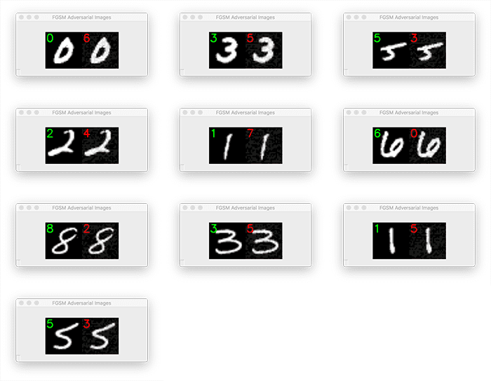
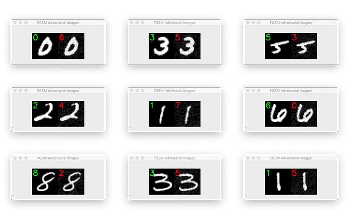
Figure 4: The results of applying adversarial image training using the FGSM. Example digits are shown before FGSM adversarial attack (green) followed by after (red). These pairs of digits are essentially identical to the human eye, but according to our CNN, are misclassified.

Figure 4 displays a montage of ten images, including the original MNIST image from the testing set (left) and the output FGSM image (right).

Visually, the adversarial FGSM images are identical to the original digit images; however, our CNN is completely fooled, making incorrect predictions for each of the images.

What’s the big deal?

Fooling a CNN using adversarial images and causing it to make incorrect predictions on the MNIST dataset seems low consequence.

But what happens if that model were trained to detect pedestrians crossing the street and deployed to a self-driving car? There would be tremendous consequences as now people’s lives would be on the line.

That raises the question:

If it’s so easy to fool CNNs, what can we do to defend against adversarial attacks?

In the next two blog posts, I’ll show you how to defend against adversarial attacks by updating our training procedure to include adversarial images.

Credits and references

The FGSM implementation was inspired by Sebastian Theiler’s excellent article on adversarial attacks and defenses. A huge shoutout and thank you to Sebastian for sharing his knowledge.

What’s next? We recommend PyImageSearch University.

Course information:
86+ total classes • 115+ hours hours of on-demand code walkthrough videos • Last updated: February 2025
★★★★★ 4.84 (128 Ratings) • 16,000+ Students Enrolled

I strongly believe that if you had the right teacher you could master computer vision and deep learning.

Do you think learning computer vision and deep learning has to be time-consuming, overwhelming, and complicated? Or has to involve complex mathematics and equations? Or requires a degree in computer science?

That’s not the case.

All you need to master computer vision and deep learning is for someone to explain things to you in simple, intuitive terms. And that’s exactly what I do. My mission is to change education and how complex Artificial Intelligence topics are taught.

If you’re serious about learning computer vision, your next stop should be PyImageSearch University, the most comprehensive computer vision, deep learning, and OpenCV course online today. Here you’ll learn how to successfully and confidently apply computer vision to your work, research, and projects. Join me in computer vision mastery.

Inside PyImageSearch University you’ll find:

• ✓ 86+ courses on essential computer vision, deep learning, and OpenCV topics
• ✓ 86 Certificates of Completion
• ✓ 115+ hours hours of on-demand video
• ✓ Brand new courses released regularly, ensuring you can keep up with state-of-the-art techniques
• ✓ Pre-configured Jupyter Notebooks in Google Colab
• ✓ Run all code examples in your web browser — works on Windows, macOS, and Linux (no dev environment configuration required!)
• ✓ Access to centralized code repos for all 540+ tutorials on PyImageSearch
• ✓ Easy one-click downloads for code, datasets, pre-trained models, etc.
• ✓ Access on mobile, laptop, desktop, etc.

Click here to join PyImageSearch University

Summary

In this tutorial, you learned how to implement the Fast Gradient Sign Method (FGSM) for adversarial image generation. We implemented FGSM using Keras and TensorFlow, but you can certainly translate the code into a deep learning library of your choosing.

The FGSM works by:

1. Taking an input image
2. Making predictions on the image using a trained CNN
3. Computing the loss of the prediction based on the true class label
4. Calculating the gradients of the loss with respect to the input image
5. Computing the sign of the gradient
6. Using the signed gradient to construct the output adversarial image

It may sound complicated, but as we saw, we were able to implement FGSM in under 30 lines of code, thanks to TensorFlow’s fantastic

GradientTape

GradientTape function, which makes gradient computation a breeze.

Now that you learned how to construct adversarial images using FGSM, you’ll learn how to defend against these attacks by incorporating adversarial images into your training process next week.

Stay tuned. You won’t want to miss this tutorial!

To download the source code to this post (and be notified when future tutorials are published here on PyImageSearch), simply enter your email address in the form below!

Download the Source Code and FREE 17-page Resource Guide

Enter your email address below to get a .zip of the code and a FREE 17-page Resource Guide on Computer Vision, OpenCV, and Deep Learning. Inside you’ll find my hand-picked tutorials, books, courses, and libraries to help you master CV and DL!