Spearman's rank correlation coefficient - Wikipedia

From Wikipedia, the free encyclopedia

Nonparametric measure of rank correlation

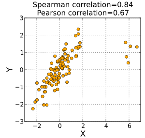
A Spearman correlation of $1$ results when the two variables being compared are monotonically related, even if their relationship is not linear. This means that all data points with greater $x$ values than that of a given data point will have greater $y$ values as well. In contrast, this does not give a perfect Pearson correlation.

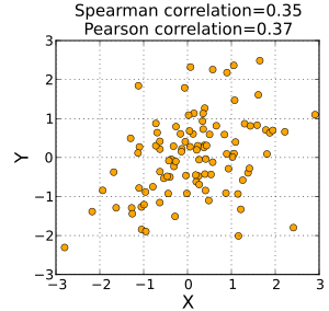
When the data are roughly elliptically distributed and there are no prominent outliers, the Spearman correlation and Pearson correlation give similar values.

The Spearman correlation is less sensitive than the Pearson correlation to strong outliers that are in the tails of both samples. That is because Spearman’s ρ limits the outlier to the value of its rank.

In statistics, Spearman’s rank correlation coefficient or Spearman’s ρ, named after Charles Spearman¹ and often denoted by the Greek letter $\rho$ (rho) or as $r_s$ , is a nonparametric measure of rank correlation (statistical dependence between the rankings of two variables). It assesses how well the relationship between two variables can be described using a monotonic function.

The Spearman correlation between two variables is equal to the Pearson correlation between the rank values of those two variables; while Pearson’s correlation assesses linear relationships, Spearman’s correlation assesses monotonic relationships (whether linear or not). If there are no repeated data values, a perfect Spearman correlation of +1 or −1 occurs when each of the variables is a perfect monotone function of the other.

Intuitively, the Spearman correlation between two variables will be high when observations have a similar (or identical for a correlation of 1) rank (i.e. relative position label of the observations within the variable: 1st, 2nd, 3rd, etc.) between the two variables, and low when observations have a dissimilar (or fully opposed for a correlation of −1) rank between the two variables.

Spearman’s coefficient is appropriate for both continuous and discrete ordinal variables.²³ Both Spearman’s $\rho$ and Kendall’s $\tau$ can be formulated as special cases of a more general correlation coefficient.

The coefficient can be used to determine how well data fits a model,⁴ like when determining the similarity of text documents.⁵

Definition and calculation

The Spearman correlation coefficient is defined as the Pearson correlation coefficient between the rank variables.⁶

For a sample of size   $n,$ the   $n$ pairs of raw scores   $\left(X_i,Y_i\right)$ are converted to ranks   $R[X_i],R[Y_i],$ and   $r_s$ is computed as

$r_s=\rho [R[X],R[Y]]=\frac{\mathrm{cov}[R[X],R[Y]]}{{\sigma }_{R[X]}{\sigma }_{R[Y]}},$

where

$\rho$ denotes the conventional Pearson correlation coefficient operator, but applied to the rank variables,

$\mathrm{cov}[R[X],R[Y]]$ is the covariance of the rank variables,

${\sigma }_{R[X]}$ and   ${\sigma }_{R[Y]}$ are the standard deviations of the rank variables.

Only when all   $n$ ranks are distinct integers (no ties), it can be computed using the popular formula

$r_s=1-\frac{6\sum d_i^2}{n\left(n^2-1\right)},$

where

$d_i\equiv R[X_i]-R[Y_i]$ is the difference between the two ranks of each observation,

  $n$ is the number of observations.

Identical values are usually⁷ each assigned fractional ranks equal to the average of their positions in the ascending order of the values, which is equivalent to averaging over all possible permutations.

If ties are present in the data set, the simplified formula above yields incorrect results: Only if in both variables all ranks are distinct, then   ${\sigma }_{R[X]}{\sigma }_{R[Y]}=$  $\mathrm{var}[R[X]]=$  $\mathrm{var}[R[Y]]=$    $\frac{1}{12}\left(n^2-1\right)$ (calculated according to biased variance). The first equation — normalizing by the standard deviation — may be used even when ranks are normalized to [0, 1] (“relative ranks”) because it is insensitive both to translation and linear scaling.

The simplified method should also not be used in cases where the data set is truncated; that is, when the Spearman’s correlation coefficient is desired for the top X records (whether by pre-change rank or post-change rank, or both), the user should use the Pearson correlation coefficient formula given above.⁸

There are several other numerical measures that quantify the extent of statistical dependence between pairs of observations. The most common of these is the Pearson product-moment correlation coefficient, which is a similar correlation method to Spearman’s rank, that measures the “linear” relationships between the raw numbers rather than between their ranks.

An alternative name for the Spearman rank correlation is the “grade correlation”;⁹ in this, the “rank” of an observation is replaced by the “grade”. In continuous distributions, the grade of an observation is, by convention, always one half less than the rank, and hence the grade and rank correlations are the same in this case. More generally, the “grade” of an observation is proportional to an estimate of the fraction of a population less than a given value, with the half-observation adjustment at observed values. Thus this corresponds to one possible treatment of tied ranks. While unusual, the term “grade correlation” is still in use.¹⁰

A positive Spearman correlation coefficient corresponds to an increasing monotonic trend between X and Y.

A negative Spearman correlation coefficient corresponds to a decreasing monotonic trend between X and Y.

The sign of the Spearman correlation indicates the direction of association between X (the independent variable) and Y (the dependent variable). If Y tends to increase when X increases, the Spearman correlation coefficient is positive. If Y tends to decrease when X increases, the Spearman correlation coefficient is negative. A Spearman correlation of zero indicates that there is no tendency for Y to either increase or decrease when X increases. The Spearman correlation increases in magnitude as X and Y become closer to being perfectly monotonic functions of each other. When X and Y are perfectly monotonically related, the Spearman correlation coefficient becomes 1. A perfectly monotonic increasing relationship implies that for any two pairs of data values X_i, Y_i and X_j, Y_j, that X_i − X_j and Y_i − Y_j always have the same sign. A perfectly monotonic decreasing relationship implies that these differences always have opposite signs.

The Spearman correlation coefficient is often described as being “nonparametric”. This can have two meanings. First, a perfect Spearman correlation results when X and Y are related by any monotonic function. Contrast this with the Pearson correlation, which only gives a perfect value when X and Y are related by a linear function. The other sense in which the Spearman correlation is nonparametric is that its exact sampling distribution can be obtained without requiring knowledge (i.e., knowing the parameters) of the joint probability distribution of X and Y.

In this example, the arbitrary raw data in the table below is used to calculate the correlation between the IQ of a person with the number of hours spent in front of TV per week [fictitious values used].

IQ, $X_i$	Hours of TV per week, $Y_i$
106	7
100	27
86	2
101	50
99	28
103	29
97	20
113	12
112	6
110	17

Firstly, evaluate $d_i^2$ . To do so use the following steps, reflected in the table below.

1. Sort the data by the first column ( $X_i$ ). Create a new column $x_i$ and assign it the ranked values 1, 2, 3, …, n.
2. Next, sort the augmented (with $x_i$ ) data by the second column ( $Y_i$ ). Create a fourth column $y_i$ and similarly assign it the ranked values 1, 2, 3, …, n.
3. Create a fifth column $d_i$ to hold the differences between the two rank columns ( $x_i$ and $y_i$ ).
4. Create one final column $d_i^2$ to hold the value of column $d_i$ squared.

IQ, $X_i$	Hours of TV per week, $Y_i$	rank $x_i$	rank $y_i$	$d_i$	$d_i^2$
86	2	1	1	0	0
97	20	2	6	−4	16
99	28	3	8	−5	25
100	27	4	7	−3	9
101	50	5	10	−5	25
103	29	6	9	−3	9
106	7	7	3	4	16
110	17	8	5	3	9
112	6	9	2	7	49
113	12	10	4	6	36

With $d_i^2$ found, add them to find $\sum d_i^2=194$ . The value of n is 10. These values can now be substituted back into the equation

$\rho =1-\frac{6\sum d_i^2}{n(n^2-1)}$

to give

$\rho =1-\frac{6\times 194}{10(10^2-1)},$

which evaluates to ρ = −29/165 = −0.175757575… with a p-value = 0.627188 (using the t-distribution).

Chart of the data presented. It can be seen that there might be a negative correlation, but that the relationship does not appear definitive.

That the value is close to zero shows that the correlation between IQ and hours spent watching TV is very low, although the negative value suggests that the longer the time spent watching television the lower the IQ. In the case of ties in the original values, this formula should not be used; instead, the Pearson correlation coefficient should be calculated on the ranks (where ties are given ranks, as described above).

Confidence intervals

Confidence intervals for Spearman’s ρ can be easily obtained using the Jackknife Euclidean likelihood approach in de Carvalho and Marques (2012).¹¹ The confidence interval with level $\alpha$ is based on a Wilks’ theorem given in the latter paper, and is given by

$\left\{\theta :\frac{\{{\sum }_{i=1}^n(Z_i-\theta ){\}}^2}{{\sum }_{i=1}^n(Z_i-\theta {)}^2}\le {\chi }_{1,\alpha }^2\right\},$

where ${\chi }_{1,\alpha }^2$ is the $\alpha$ quantile of a chi-square distribution with one degree of freedom, and the $Z_i$ are jackknife pseudo-values. This approach is implemented in the R package spearmanCI.

Determining significance

One approach to test whether an observed value of ρ is significantly different from zero (r will always maintain −1 ≤ r ≤ 1) is to calculate the probability that it would be greater than or equal to the observed r, given the null hypothesis, by using a permutation test. An advantage of this approach is that it automatically takes into account the number of tied data values in the sample and the way they are treated in computing the rank correlation.

Another approach parallels the use of the Fisher transformation in the case of the Pearson product-moment correlation coefficient. That is, confidence intervals and hypothesis tests relating to the population value ρ can be carried out using the Fisher transformation:

$F(r)=\frac{1}{2}\ln \frac{1+r}{1-r}=\mathrm{arctanh}r.$

If F(r) is the Fisher transformation of r, the sample Spearman rank correlation coefficient, and n is the sample size, then

$z=\sqrt{\frac{n-3}{1.06}}F(r)$

is a z-score for r, which approximately follows a standard normal distribution under the null hypothesis of statistical independence (ρ = 0).¹²¹³

One can also test for significance using

$t=r\sqrt{\frac{n-2}{1-r^2}},$

which is distributed approximately as Student’s t-distribution with n − 2 degrees of freedom under the null hypothesis.¹⁴ A justification for this result relies on a permutation argument.¹⁵

A generalization of the Spearman coefficient is useful in the situation where there are three or more conditions, a number of subjects are all observed in each of them, and it is predicted that the observations will have a particular order. For example, a number of subjects might each be given three trials at the same task, and it is predicted that performance will improve from trial to trial. A test of the significance of the trend between conditions in this situation was developed by E. B. Page¹⁶ and is usually referred to as Page’s trend test for ordered alternatives.

Correspondence analysis based on Spearman’s ρ

Classic correspondence analysis is a statistical method that gives a score to every value of two nominal variables. In this way the Pearson correlation coefficient between them is maximized.

There exists an equivalent of this method, called grade correspondence analysis, which maximizes Spearman’s ρ or Kendall’s τ.¹⁷

Approximating Spearman’s ρ from a stream

There are two existing approaches to approximating the Spearman’s rank correlation coefficient from streaming data.¹⁸¹⁹ The first approach¹⁸ involves coarsening the joint distribution of $(X,Y)$ . For continuous $X,Y$ values: $m_1,m_2$ cutpoints are selected for $X$ and $Y$ respectively, discretizing these random variables. Default cutpoints are added at $-\infty$ and $\infty$ . A count matrix of size $(m_1+1)\times (m_2+1)$ , denoted $M$ , is then constructed where $M[i,j]$ stores the number of observations that fall into the two-dimensional cell indexed by $(i,j)$ . For streaming data, when a new observation arrives, the appropriate $M[i,j]$ element is incremented. The Spearman’s rank correlation can then be computed, based on the count matrix $M$ , using linear algebra operations (Algorithm 2¹⁸). Note that for discrete random variables, no discretization procedure is necessary. This method is applicable to stationary streaming data as well as large data sets. For non-stationary streaming data, where the Spearman’s rank correlation coefficient may change over time, the same procedure can be applied, but to a moving window of observations. When using a moving window, memory requirements grow linearly with chosen window size.

The second approach to approximating the Spearman’s rank correlation coefficient from streaming data involves the use of Hermite series based estimators.¹⁹ These estimators, based on Hermite polynomials, allow sequential estimation of the probability density function and cumulative distribution function in univariate and bivariate cases. Bivariate Hermite series density estimators and univariate Hermite series based cumulative distribution function estimators are plugged into a large sample version of the Spearman’s rank correlation coefficient estimator, to give a sequential Spearman’s correlation estimator. This estimator is phrased in terms of linear algebra operations for computational efficiency (equation (8) and algorithm 1 and 2¹⁹). These algorithms are only applicable to continuous random variable data, but have certain advantages over the count matrix approach in this setting. The first advantage is improved accuracy when applied to large numbers of observations. The second advantage is that the Spearman’s rank correlation coefficient can be computed on non-stationary streams without relying on a moving window. Instead, the Hermite series based estimator uses an exponential weighting scheme to track time-varying Spearman’s rank correlation from streaming data, which has constant memory requirements with respect to “effective” moving window size. A software implementation of these Hermite series based algorithms exists ²⁰ and is discussed in Software implementations.

Software implementations

• R’s statistics base-package implements the test cor.test(x, y, method = "spearman") in its “stats” package (also cor(x, y, method = "spearman") will work. The package spearmanCI computes confidence intervals. The package hermiter²⁰ computes fast batch estimates of the Spearman correlation along with sequential estimates (i.e. estimates that are updated in an online/incremental manner as new observations are incorporated).

• Stata implementation: spearman *varlist* calculates all pairwise correlation coefficients for all variables in varlist.

• MATLAB implementation: [r,p] = corr(x,y,'Type','Spearman') where r is the Spearman’s rank correlation coefficient, p is the p-value, and x and y are vectors.²¹

• Python has many different implementations of the spearman correlation statistic: it can be computed with the spearmanr function of the scipy.stats module, as well as with the DataFrame.corr(method='spearman') method from the pandas library, and the corr(x, y, method='spearman') function from the statistical package pingouin.

• Kendall tau rank correlation coefficient

• Chebyshev’s sum inequality, rearrangement inequality (These two articles may shed light on the mathematical properties of Spearman’s ρ.)

• Distance correlation

• Polychoric correlation

• Corder, G. W. & Foreman, D. I. (2014). Nonparametric Statistics: A Step-by-Step Approach, Wiley. ISBN 978-1118840313.

• Daniel, Wayne W. (1990). “Spearman rank correlation coefficient”. Applied Nonparametric Statistics (2nd ed.). Boston: PWS-Kent. pp. 358–365. ISBN 978-0-534-91976-4.

• Spearman C. (1904). “The proof and measurement of association between two things”. American Journal of Psychology. 15 (1): 72–101. doi:10.2307/1412159. JSTOR 1412159.

• Bonett D. G., Wright, T. A. (2000). “Sample size requirements for Pearson, Kendall, and Spearman correlations”. Psychometrika. 65: 23–28. doi:10.1007/bf02294183. S2CID 120558581.{{[cite journal](https://en.wikipedia.org/wiki/Template:Cite_journal "Template:Cite journal")}}: CS1 maint: multiple names: authors list (link)

• Kendall M. G. (1970). Rank correlation methods (4th ed.). London: Griffin. ISBN 978-0-852-6419-96. OCLC 136868.

• Hollander M., Wolfe D. A. (1973). Nonparametric statistical methods. New York: Wiley. ISBN 978-0-471-40635-8. OCLC 520735.

• Caruso J. C., Cliff N. (1997). “Empirical size, coverage, and power of confidence intervals for Spearman’s Rho”. Educational and Psychological Measurement. 57 (4): 637–654. doi:10.1177/0013164497057004009. S2CID 120481551.

• Table of critical values of ρ for significance with small samples

• Spearman’s Rank Correlation Coefficient – Excel Guide: sample data and formulae for Excel, developed by the Royal Geographical Society.

Footnotes

1. Spearman, C. (January 1904). “The Proof and Measurement of Association between Two Things” (PDF). The American Journal of Psychology. 15 (1): 72–101. doi:10.2307/1412159. JSTOR 1412159. ↩

2. Scale types. ↩

3. Lehman, Ann (2005). Jmp For Basic Univariate And Multivariate Statistics: A Step-by-step Guide. Cary, NC: SAS Press. p. 123. ISBN 978-1-59047-576-8. ↩

4. Royal Geographic Society. “A Guide to Spearman’s Rank” (PDF). ↩

5. Nino Arsov; Milan Dukovski; Milan Dukovski; Blagoja Evkoski (November 2019). “A Measure of Similarity in Textual Data Using Spearman’s Rank Correlation Coefficient”. ↩

6. Myers, Jerome L.; Well, Arnold D. (2003). Research Design and Statistical Analysis (2nd ed.). Lawrence Erlbaum. pp. 508. ISBN 978-0-8058-4037-7. ↩

7. Dodge, Yadolah, ed. (2010). The Concise Encyclopedia of Statistics. New York, NY: Springer-Verlag. p. 502. ISBN 978-0-387-31742-7. ↩

8. al Jaber, Ahmed Odeh; Elayyan, Haifaa Omar (2018). Toward Quality Assurance and Excellence in Higher Education. River Publishers. p. 284. ISBN 978-87-93609-54-9. ↩

9. Yule, G. U.; Kendall, M. G. (1968) [1950]. An Introduction to the Theory of Statistics (14th ed.). Charles Griffin & Co. p. 268. ↩

10. Piantadosi, J.; Howlett, P.; Boland, J. (2007). “Matching the grade correlation coefficient using a copula with maximum disorder”. Journal of Industrial and Management Optimization. 3 (2): 305–312. doi:10.3934/jimo.2007.3.305. ↩

11. de Carvalho, M.; Marques, F. (2012). “Jackknife Euclidean likelihood-based inference for Spearman’s rho” (PDF). North American Actuarial Journal. 16 (4): 487‒492. doi:10.1080/10920277.2012.10597644. S2CID 55046385. ↩

12. Choi, S. C. (1977). “Tests of Equality of Dependent Correlation Coefficients”. Biometrika. 64 (3): 645–647. doi:10.1093/biomet/64.3.645. ↩

13. Fieller, E. C.; Hartley, H. O.; Pearson, E. S. (1957). “Tests for rank correlation coefficients. I”. Biometrika. 44 (3–4): 470–481. CiteSeerX 10.1.1.474.9634. doi:10.1093/biomet/44.3-4.470. ↩

14. Press; Vettering; Teukolsky; Flannery (1992). Numerical Recipes in C: The Art of Scientific Computing (2nd ed.). Cambridge University Press. p. 640. ISBN 9780521437202. ↩

15. Kendall, M. G.; Stuart, A. (1973). “Sections 31.19, 31.21”. The Advanced Theory of Statistics, Volume 2: Inference and Relationship. Griffin. ISBN 978-0-85264-215-3. ↩

16. Page, E. B. (1963). “Ordered hypotheses for multiple treatments: A significance test for linear ranks”. Journal of the American Statistical Association. 58 (301): 216–230. doi:10.2307/2282965. JSTOR 2282965. ↩

17. Kowalczyk, T.; Pleszczyńska, E.; Ruland, F., eds. (2004). Grade Models and Methods for Data Analysis with Applications for the Analysis of Data Populations. Studies in Fuzziness and Soft Computing. Vol. 151. Berlin Heidelberg New York: Springer Verlag. ISBN 978-3-540-21120-4. ↩

18. Xiao, W. (2019). “Novel Online Algorithms for Nonparametric Correlations with Application to Analyze Sensor Data”. 2019 IEEE International Conference on Big Data (Big Data). pp. 404–412. doi:10.1109/BigData47090.2019.9006483. ISBN 978-1-7281-0858-2. S2CID 211298570. ↩ ↩² ↩³

19. Stephanou, Michael; Varughese, Melvin (July 2021). “Sequential estimation of Spearman rank correlation using Hermite series estimators”. Journal of Multivariate Analysis. 186: 104783. arXiv:2012.06287. doi:10.1016/j.jmva.2021.104783. S2CID 235742634. ↩ ↩² ↩³

20. Stephanou, M. and Varughese, M (2023). “Hermiter: R package for sequential nonparametric estimation”. Computational Statistics. 39 (3): 1127–1163. arXiv:2111.14091. doi:10.1007/s00180-023-01382-0. S2CID 244715035.{{[cite journal](https://en.wikipedia.org/wiki/Template:Cite_journal "Template:Cite journal")}}: CS1 maint: multiple names: authors list (link) ↩ ↩²

21. “Linear or rank correlation - MATLAB corr”. www.mathworks.com. ↩