Self-Supervised Visual Representation Learning
This post consolidates several literature summaries from the field of self-supervised visual representation learning.
- MoCo: Momentum Contrast for Unsupervised Visual Representation Learning
- SimSiam: Exploring Simple Siamese Representation Learning
- BYOL: Bootstrap Your Own Latent A New Approach to Self-Supervised Learning
- UVC: Joint-task Self-supervised Learning for Temporal Correspondence
- SwAV: Unsupervised Learning of Visual Features by Contrasting Cluster Assignments
- VFS: Rethinking Self-supervised Correspondence Learning A Video Frame-level Similarity Perspective
MoCo: Momentum Contrast for Unsupervised Visual Representation Learning
Notes on MoCo: Momentum Contrast for Unsupervised Visual Representation Learning by Kaiming He and colleagues.
Abstract broken up with some added emphasis:
We present Momentum Contrast (MoCo) for unsupervised visual representation learning. From a perspective on contrastive learning [29] as dictionary look-up, we build a dynamic dictionary with a queue and a moving-averaged encoder. This enables building a large and consistent dictionary on-the-fly that facilitates contrastive unsupervised learning.
MoCo provides competitive results under the common linear protocol on ImageNet classification.
More importantly, the representations learned by MoCo transfer well to downstream tasks. MoCo can outperform its supervised pre-training counterpart in 7 detection/segmentation tasks on PASCAL VOC, COCO, and other datasets, sometimes surpassing it by large margins.
This suggests that the gap between unsupervised and supervised representation learning has been largely closed in many vision tasks.
Introduction
Authors state the continuous signal space of computer vision makes it less amenable to self-supervised techniques as compared to NLP, whose samples are constituted of token form a finite signal space, concretely of the vocabulary size:
The reason may stem from differences in their respective signal spaces. Language tasks have discrete signal spaces (words, sub-word units, etc.) for building tokenized dictionaries, on which unsupervised learning can be based. Computer vision, in contrast, further concerns dictionary building [54, 9, 5], as the raw signal is in a continuous, high-dimensional space and is not structured for human communication (e.g., unlike words)
They frame contrastive learning in terms of dictionary look-up against dynamic dictionaries:
[Contrastive learning] can be thought of as building dynamic dictionaries. The “keys” (tokens) in the dictionary are sampled from data (e.g., images or patches) and are represented by an encoder network. Unsupervised learning trains encoders to perform dictionary look-up: an encoded “query” should be similar to its matching key and dissimilar to others. Learning is formulated as minimizing a contrastive loss1
They target having dictionaries (for looking up query image views against) that are:
- Large
- Consistent as they evolve (see [#inconsistency-of-encoded-representations])
- The momentum contrast dictionary is a queue of data samples, where the latest minibatch is enqueued and the oldest is dequeued.
- This decouples the dictionary size from the batch size.
- The key encoder for encoding the dictionary entries (samples) is a momentum-based moving average of the query encoder, proposed to maintain consistency of the keys against which new samples are queried in the contrastive loss.
Et voilà, MoCo 😉
Interestingly, it is appropriate to think of MoCo as a way of building dynamic dictionaries for any kind of contrastive learning, so you can swap out different pretext tasks:
MoCo is a mechanism for building dynamic dictionaries for contrastive learning, and can be used with various pretext tasks. In this paper, we follow a simple instance discrimination task [61, 63, 2]: a query matches a key if they are encoded views (e.g., different crops) of the same image.
As we know with self-supervised learning, we have pretext tasks + loss functions:
self-supervised learning methods generally involve two aspects: pretext tasks and loss functions.
The term “pretext” implies that the task being solved is not of genuine interest, but is solved only for the true purpose of learning a good data representation.
Loss functions can often be investigated independently of pretext tasks. MoCo focuses on the loss function aspect.
Contrastive Learning as Dictionary Look-up
The authors use the InfoNCE loss:
\[\mathcal{L}_{q}=-\log \frac{\exp \left(q \cdot k_{+} / \tau\right)}{\sum_{i=0}^{K} \exp \left(q \cdot k_{i} / \tau\right)}\]As can be seen, this is a simple negative log-softmax where the correct class is the positive key, $k_+$, and the denominator indexes over all keys in the dictionary.
Additionally, a temperature hyperparameter, $\tau$, is used for tuning. Using a high temperature makes the probability distribution more diffuse across classes (i.e. ‘softer’) and means we obtain predictions with higher uncertainty. Conversely, using a low temperature makes the probability distribution ‘harder’, reducing uncertainty of the predictions; setting $\tau = 1$ of course reduces this to the regular (negative log-)softmax. (Temperature as a softmax hyperparameter is explained here and demonstrated practically in this post.)
Keep in mind, contrastive losses can be based on margins (e.g. based on hinge loss for positive and negative samples) or other variants of NCE losses.
Key Ideas: Momentum and the Queue of Keys
I added numbers (1) and (2) to the extract below to emphasise MoCo’s two main conributions:
- Use momentum (an exponential moving average) to update the key encoder on the basis of the current iteration’s query encoder and (a weighted combination of) past iterations’ query parameters.
- Use a queue to keep the negative samples for a additional, manageable memory overhead that enables use of a larger range of negative samples.

Figure 1. Momentum Contrast (MoCo) trains a visual representation encoder by matching an encoded query $q$ to a dictionary of encoded keys using a contrastive loss. The dictionary keys $\{k0, k1, k2, \dots \}$ are defined on-the-fly by a set of data samples.
The dictionary is built as a queue, with the current mini-batch enqueued and the oldest mini-batch dequeued, decoupling it from the mini-batch size.
The keys are encoded by a slowly progressing encoder, driven by a momentum update with the query encoder. This method enables a large and consistent dictionary for learning visual representations.
Algorithm

The above is the algorithm for MoCo.
We initialise the parameters of the key encoder as the same randomly initialised parameters as the query encoder.
Then for each minibatch:
- Create two randomly augmented versions of the input images (in current minibatch)
- Run the forward pass of the query image(s) through the query encoder and key image(s) through the key encoder
- Calculate positive logit(s)2 which come from the matrix multiplication of the query and key image(s)
- NOTE: If the batch size were 1, there would be only 1 positive logit corresponding to the positive sample
- Calculate negative logits which come from the matrix multiplication of the query and queue images
- Concatenate the positive and negative logits
- Compute the contrastive InfoNCE loss as the softmax shown before
- in the algorithm, they use the label vector as an $N$-dimensional vector of zeros since they put the positive logit in the first position via
cat[l_pos, l_neg], dim=1)
- in the algorithm, they use the label vector as an $N$-dimensional vector of zeros since they put the positive logit in the first position via
- Backpropagate gradients
- Update the query encoder parameters only via the optimiser (using the computed gradients)
- Update the key encoder via a momentum (exponential moving average) update: $\theta_\text{key} = m \cdot \theta_\text{key} + (m - 1) \cdot \theta_\text{query}$ where they use $m=0.999$ (see Implementation)
- This places most of the weight for the update on parameter values from previous iterations, but still allows more recent iterations to contribute significantly over the course of e.g. an epoch
Shuffling Batch Norm: Batch Normalisation Leaking Information
The authors shuffle batch normalisation in order to prevent the model from using BN layers to exploit information across batches to decrease the loss on the pretext task without improving the quality (downstream performance) of the learnt encoder.
This happens because performing batch norm leaks mean and variance statistics across batches, allowing the model to set the $\alpha$ and $\beta$ learn parameters of the BN layer to better fit the training data better in a trivial fashion.
Shuffling BN. Our encoders $f_q$ and $f_k$ both have Batch Normalization (BN) [37] as in the standard ResNet [33]. In experiments, we found that using BN prevents the model from learning good representations, as similarly reported in [35] (which avoids using BN). The model appears to “cheat” the pretext task and easily finds a low-loss solution. This is possibly because the intra-batch communication among samples (caused by BN) leaks information.
Specifically, the condition they satisfy is:
[ensuring] the batch statistics used to compute a query and its positive key come from two different [data] subsets. This effectively tackles the cheating issue and allows training to benefit from BN.
The way they do this is fiddly:
We resolve this problem by shuffling BN. We train with multiple GPUs and perform BN on the samples independently for each GPU (as done in common practice). For the key encoder $f_k$, we shuffle the sample order in the current mini-batch before distributing it among GPUs (and shuffle back after encoding); the sample order of the mini-batch for the query encoder $f_q$ is not altered.
The SSL set-up that uses a memory bank (one of the two previous self-supervised set-ups they compare against) doesn’t suffer from this information leakage problem since the positive keys are from different, previous batches.
What is the Dictionary Queue
MoCo uses a queue to represent the dictionary of keys that make up negative samples to contrast the positive augmented sample against; when putting the query through the contrastive loss.
How does the dictionary queue work? Implementation
The dictionary is implemented as a queue.
Specifically, in the PyTorch implementation, in the MoCo class __init__ body, they:
- register a buffer (see What is a buffer in PyTorch) of dimension (feature dimension $\times$ queue size), randomly initialised to use as a queue
- register another buffer to use as a pointer for the queue
def __init__(self, base_encoder, dim=128, K=65536, m=0.999, T=0.07, mlp=False):
    '''
    dim: feature dimension (default: 128)
    K: queue size; number of negative keys (default: 65536)
    '''

    # ...

    # create the queue
    self.register_buffer("queue", torch.randn(dim, K))
    self.queue = nn.functional.normalize(self.queue, dim=0)

    self.register_buffer("queue_ptr", torch.zeros(1, dtype=torch.long))
Then, they have a method (decorated with @torch.no_grad()) that they call at the end of every iteration, i.e. at the end of the forward pass.
They pass k the encoded keys to the function to “enqueue” them, whilst “dequeuing” the oldest ones, which they track by moving the queue pointer along by the batch size each time: ptr = (ptr + batch_size) % self.K # move pointer. As we can see, there’s no actual enqueuing and dequeuing happening, and instead by using a pointer they just directly replace the oldest (encoded) keys with the new batch of (encoded) keys.
@torch.no_grad()
def _dequeue_and_enqueue(self, keys):
    # gather keys before updating queue
    keys = concat_all_gather(keys)

    batch_size = keys.shape[0]

    ptr = int(self.queue_ptr)
    assert self.K % batch_size == 0  # for simplicity

    # replace the keys at ptr (dequeue and enqueue)
    self.queue[:, ptr:ptr + batch_size] = keys.T
    ptr = (ptr + batch_size) % self.K  # move pointer

    self.queue_ptr[0] = ptr
So basically, as is evident from the above, the added memory overhead is an additional Tensor of size dim by K. Given that When PyTorch is initialized its default floating point dtype is torch.float32 (mentioned at the torch.set_default_dtype) docs), which is a 32-bit floating point, we have a memory overhead of:
- 32 bits $\times$ dim $\times$ K
- For default values of $128 = 2^7$ and $65536 = 2^{16}$ we have:
- $32 \times 128 \times 65536 = 2^5 \cdot 2^7 \cdot 2^{16} = 2^{28} = 268435456$ bits
- $= 2^{25} = 33554432$ bytes
- or $\approx 33.5$ MB
What is a buffer in PyTorch
A Module buffer is a Tensor attribute of a Module that is not a model Parameter
See the register_buffer method in the docs for Module:
Adds a buffer to the module.
This is typically used to register a buffer that should not to be considered a model parameter. For example, BatchNorm’s running_mean is not a parameter, but is part of the module’s state. Buffers, by default, are persistent and will be saved alongside parameters. This behavior can be changed by setting persistent to False. The only difference between a persistent buffer and a non-persistent buffer is that the latter will not be a part of this module’s state_dict.
Buffers can be accessed as attributes using given names.
Details
- Remember to always take the (e.g. L2) norm of the feature representation of an image returned by the encoder to put it into a contrastive loss.
Comparison to Previous Self-Supervised Approaches

In comparison to previous approaches, you
- Don’t have this issue of inconsistent key representations during training when you do the update with gradients
- this corresponds to the end-to-end model (a) pictured above
- Don’t require a heavy memory bank
- this is (b) as devised in Unsupervised Feature Learning via Non-Parametric Instance Discrimination by Zhirong Wu and colleagues from 2018
Inconsistency of encoded representations
Why Was MoCo Proposed? The following sets the ground for part of the reason why MoCo was necessary given the context of SimCLR being the prevailing / landmark self-supervised visual representation learning.
It is taken from Understanding Contrastive Learning and MoCo: What is important in contrastive learning and how it can help by Shuchen Du:
Inconsistency of encoded representations
In SimCLR, we have only one encoder through which a mini-batch is passed then positive and negative pairs are constructed for training. In this way, positive and negative pairs are consistent, which means they are generated from an encoder with the same parameters. On the other hand, the parameters of the encoder are not changed during the generation of all pair data in a mini-batch. That is important because the parameters of the encoder are updated per mini-batch, thus for the same input image, the generated representations will be different from different mini-batches. This phenomenon is called inconsistent representation generation. Since the encoder is updated every mini-batch, the generated representations in current mini-batch will be getting ‘old’ compared to those generated in the future mini-batches. Therefore, it is not optimal to mix representations from different mini-batches and use them together during training. It is also the reason why SimCLR uses large batch sizes.
Before MoCo is proposed, people tend to use a memory bank to keep a large amount of inconsistent representations to meet the demand of large amount of negative pair constructions. However, the performance is not good due to the sub-optimal inconsistent representations. Therefore, MoCo is proposed to convert the representations encoded from different mini-batches from inconsistency to consistency.
As the authors say themselves in the text (see Introduction):
…while the keys in the dictionary should be represented by the same or similar encoder so that their comparisons to the query are consistent.
Implementation
For concreteness, here is the implementation of the MoCo class as a torch.nn.Module.
Up top, we can see that they use default values of
- Very large momentum value, $m = 0.999$, so that the key encoder network’s parameters are basically constant, instead of updated each minibatch like in previous work (e.g. SimCLR) with a small contribution from the current iteration’s parameter values.
- Of course over the course of an epoch, this relative weighting in the EMA will lead to significant contributions from up-to-date iterations
- Temperature of 0.07 which is a common choice
- Key queue size of $65,536 = 2^{16}$ (probably a power of two to fit nicely into memory on the even number of GPUs)
In the initialisation method arguments, we have the defaults:
K=65536, m=0.999, T=0.07
import torch
import torch.nn as nn


class MoCo(nn.Module):
    """
    Build a MoCo model with: a query encoder, a key encoder, and a queue
    https://arxiv.org/abs/1911.05722
    """
    def __init__(self, base_encoder, dim=128, K=65536, m=0.999, T=0.07, mlp=False):
        """
        dim: feature dimension (default: 128)
        K: queue size; number of negative keys (default: 65536)
        m: moco momentum of updating key encoder (default: 0.999)
        T: softmax temperature (default: 0.07)
        """
        super(MoCo, self).__init__()

        self.K = K
        self.m = m
        self.T = T

        # create the encoders
        # num_classes is the output fc dimension
        self.encoder_q = base_encoder(num_classes=dim)
        self.encoder_k = base_encoder(num_classes=dim)

        if mlp:  # hack: brute-force replacement
            dim_mlp = self.encoder_q.fc.weight.shape[1]
            self.encoder_q.fc = nn.Sequential(nn.Linear(dim_mlp, dim_mlp),
                                              nn.ReLU(),
                                              self.encoder_q.fc)
            self.encoder_k.fc = nn.Sequential(nn.Linear(dim_mlp, dim_mlp),
                                              nn.ReLU(),
                                              self.encoder_k.fc)

        for param_q, param_k in zip(self.encoder_q.parameters(), self.encoder_k.parameters()):
            param_k.data.copy_(param_q.data)  # initialize
            param_k.requires_grad = False  # not update by gradient

        # create the queue
        self.register_buffer("queue", torch.randn(dim, K))
        self.queue = nn.functional.normalize(self.queue, dim=0)

        self.register_buffer("queue_ptr", torch.zeros(1, dtype=torch.long))

    @torch.no_grad()
    def _momentum_update_key_encoder(self):
        """
        Momentum update of the key encoder
        """
        for param_q, param_k in zip(self.encoder_q.parameters(), self.encoder_k.parameters()):
            param_k.data = param_k.data * self.m + param_q.data * (1. - self.m)

    @torch.no_grad()
    def _dequeue_and_enqueue(self, keys):
        # gather keys before updating queue
        keys = concat_all_gather(keys)

        batch_size = keys.shape[0]

        ptr = int(self.queue_ptr)
        assert self.K % batch_size == 0  # for simplicity

        # replace the keys at ptr (dequeue and enqueue)
        self.queue[:, ptr:ptr + batch_size] = keys.T
        ptr = (ptr + batch_size) % self.K  # move pointer

        self.queue_ptr[0] = ptr

    @torch.no_grad()
    def _batch_shuffle_ddp(self, x):
        """
        Batch shuffle, for making use of BatchNorm.
        *** Only support DistributedDataParallel (DDP) model. ***
        """
        # gather from all gpus
        batch_size_this = x.shape[0]
        x_gather = concat_all_gather(x)
        batch_size_all = x_gather.shape[0]

        num_gpus = batch_size_all // batch_size_this

        # random shuffle index
        idx_shuffle = torch.randperm(batch_size_all).cuda()

        # broadcast to all gpus
        torch.distributed.broadcast(idx_shuffle, src=0)

        # index for restoring
        idx_unshuffle = torch.argsort(idx_shuffle)

        # shuffled index for this gpu
        gpu_idx = torch.distributed.get_rank()
        idx_this = idx_shuffle.view(num_gpus, -1)[gpu_idx]

        return x_gather[idx_this], idx_unshuffle

    @torch.no_grad()
    def _batch_unshuffle_ddp(self, x, idx_unshuffle):
        """
        Undo batch shuffle.
        *** Only support DistributedDataParallel (DDP) model. ***
        """
        # gather from all gpus
        batch_size_this = x.shape[0]
        x_gather = concat_all_gather(x)
        batch_size_all = x_gather.shape[0]

        num_gpus = batch_size_all // batch_size_this

        # restored index for this gpu
        gpu_idx = torch.distributed.get_rank()
        idx_this = idx_unshuffle.view(num_gpus, -1)[gpu_idx]

        return x_gather[idx_this]

    def forward(self, im_q, im_k):
        """
        Input:
            im_q: a batch of query images
            im_k: a batch of key images
        Output:
            logits, targets
        """

        # compute query features
        q = self.encoder_q(im_q)  # queries: NxC
        q = nn.functional.normalize(q, dim=1)

        # compute key features
        with torch.no_grad():  # no gradient to keys
            self._momentum_update_key_encoder()  # update the key encoder

            # shuffle for making use of BN
            im_k, idx_unshuffle = self._batch_shuffle_ddp(im_k)

            k = self.encoder_k(im_k)  # keys: NxC
            k = nn.functional.normalize(k, dim=1)

            # undo shuffle
            k = self._batch_unshuffle_ddp(k, idx_unshuffle)

        # compute logits
        # Einstein sum is more intuitive
        # positive logits: Nx1
        l_pos = torch.einsum('nc,nc->n', [q, k]).unsqueeze(-1)
        # negative logits: NxK
        l_neg = torch.einsum('nc,ck->nk', [q, self.queue.clone().detach()])

        # logits: Nx(1+K)
        logits = torch.cat([l_pos, l_neg], dim=1)

        # apply temperature
        logits /= self.T

        # labels: positive key indicators
        labels = torch.zeros(logits.shape[0], dtype=torch.long).cuda()

        # dequeue and enqueue
        self._dequeue_and_enqueue(k)

        return logits, labels


# utils
@torch.no_grad()
def concat_all_gather(tensor):
    """
    Performs all_gather operation on the provided tensors.
    *** Warning ***: torch.distributed.all_gather has no gradient.
    """
    tensors_gather = [torch.ones_like(tensor)
        for _ in range(torch.distributed.get_world_size())]
    torch.distributed.all_gather(tensors_gather, tensor, async_op=False)

    output = torch.cat(tensors_gather, dim=0)
    return output
SimSiam: Exploring Simple Siamese Representation Learning
Notes on SimSiam: Exploring Simple Siamese Representation Learning by Xinlei and Chen Kaiming He.
- Paper: https://arxiv.org/pdf/2011.10566.pdf
- Code: https://github.com/facebookresearch/simsiam
- Papers with Code: https://paperswithcode.com/paper/exploring-simple-siamese-representation
The background and perspectives work this paper provides is a treasure trove. The point of the paper is, in many ways, to unify the perspectives brought to the table by a selection of landmark SSL vision papers (from large organisations), in particular SimCLR, MoCo, SwAV and BYOL.
Key Points
Abstract restructured
Siamese networks have become a common structure in various recent models for unsupervised visual representation learning. These models maximize the similarity between two augmentations of one image, subject to certain conditions for avoiding collapsing solutions.
In this paper, we report surprising empirical results that simple Siamese networks can learn meaningful representations even using none of the following:
- negative sample pairs
- large batches
- momentum encoders
Our experiments show that collapsing solutions do exist for the loss and structure, but a stop-gradient operation plays an essential role in preventing collapsing.
We provide a hypothesis on the implication of stop-gradient, and further show proof-of-concept experiments verifying it.
Our “SimSiam” method achieves competitive results on ImageNet and downstream tasks.
We hope this simple baseline will motivate people to rethink the roles of Siamese architectures for unsupervised representation learning.
Background and Lead-in
- Siamese networks are parallel networks with weight sharing, so can be more practically thought of as training set-ups / paradigms where the forward pass is conducted twice with different inputs, whether these come from the same image as two different “views” (also called “augmentations” or “transformations”) or different inputs (as in the supervised setting).
- They are used for comparing entities and are used for signature and face verification, tracking, one-shot learning with inputs usually being different images and supervision used for training.
- Siamese networks are used for contrastive learning where a contrastive loss attracts similar samples and repels dissimilar ones, which can in turn be used for SSL when the positive samples are from the same image and negative samples from different images. (Not just images.)
- Clustering-based methods alternate between cluster assignment of samples to act as pseudolabels, and training using those assignments.
- SwAV does clustering with a Siamese Network where one forward pass computes the cluster assignment and the other pass predicts the assignment from another view (we say predicts because that other view is given the features, and the loss is taken between cluster assignments and features, at least from what I understand of the paper at this point)
- SwAV does this online - i.e. does not alternate between cluster assignment and training with cluster pseudolabels by satisfying an equipartition constraint within batches (so batches need to be big enough, e.g. 256; or else using information from previous batches / iterations)
- SwAV solves the equipartition constraint (i.e. the transportation polytope) via the Sinkhorn-Knopp transform (see Sinkhorn Distances: Lightspeed Computation of Optimal Transport by Marco Cuturi published in 2013 at NIPS)
- Clustering-based SSL methods use clusters as negative prototypes instead of explicitly using negative samples
- Clustering-based SSL methods require large batches, a memory bank or a queue to provide enough (negative) samples for clustering
- BYOL directly predicts the output of one view from another view using a momentum encoder for one branch, which the authors hypothesise is important to avoid collapse3
Contributions
- The authors find that the momentum-encoder is not required to avoid collapse but rather a stop-gradient, which is confounded with the momentum-encoder since a stop-gradient is required for one4
- Note: A momentum-encoder might still improve accuracy for a correctly-tuned momentum value, $m$
Method
- Take two randomly augmented views, $x_1$ and $x_2$, from an image $x$
- Pass these two views through the forward pass of an encoder and projection head (e.g. ResNet followed by MLP)
- The encoder, $f$, implements weight sharing
- A projection head, $h$ transforms the output of one view and matches it to another view
- We have the two outputs from the input views: $p_1 \triangleq h(f(x_1)) \triangleq h(z_1)$ and $z_2 = f(x_2)$
- The negative cosine similarity is used as a minimisation criterion, which is equivalent to the MSE of the $\mathcal{l}_2$-normalised vectors up to a scaling coefficient of 2
- The overall loss is a “symmetrized loss” composed of the average of the two negative cosine similaries that take the output with and without the projection head (i.e. from the two branches of the network) in each case
- The average loss is taken over the images (in a minibatch) with the minimum possible loss being $-1$
**The crucial stop-gradient operation operation is implemented by modifying the negative cosine similarity function to:
\[\mathbf{\mathcal{D}(p_1, \operatorname{stopgrad}(z_2))}\]This means that $z_2$ is treated as a constant in this term
In other words, no gradient flows back from $z_2$ in this component of the loss (in the full loss, there is also the other component). The overall, stop-gradient-modified loss is:
\[\mathcal{L} = \frac{1}{2} \mathcal{D}(p_1, \operatorname{stopgrad}(z_2)) + \frac{1}{2} \mathcal{D}(p_2, \operatorname{stopgrad}(z_1)\]Keep in mind that $z_\text{view_idx}$ stands for the network output without (or I guess “before”) the projection head and $p_\text{view_idx}$ stands for the network output with the projection head.
So we have no gradient backpropagation from the no-MLP (pre-projection) output in the first term and no gradient backpropagation from the no-MLP output in the second term. Note: In this set-up, we’re always stopping the gradient flowing back from the pre-projection vectors outputs of the network.

Details
- SGD - they don’t used LARS
- SGD momentum is 0.9
- Learning Rate = Batch Size / 256 (linear scaling) with base learning rate of $0.05$.
- Learning rate has cosine decay schedule
- Weight decay is
1e-4or $10^{-4}$
- Batch size is 512 by default (using 8 GPUs), but you can vary it
- They use Batch Normalisation synchronised across devices
- Projection MLP, which is part of $f$, is a three-layer MLP (hidden FC is 2048-D) with BN each layer and ReLU apart from the output layer
- Prediction MLP, $h$, is a two-layer MLP with BN on all hidden layers except the output, which also doesn’t have a ReLU
- Input and output dimensions are equal at 2048
- Hidden layer dimension is 512
- ResNet-50 is the default backbone
- 100 epoch pretraining is reported for ablations
- Self-supervised pretraining on 1,000-class ImageNet training without labels
- Linear evaluation protocol used; this is used on validation set
- this is the same evaluation protocol everyone uses and reports e.g. SwAV
Note: $h$ is a bottleneck structure since its hidden layer dimension is 512 versus the input and output dimensionalities of 2048.
Stop-gradient

Above is Figure 2 from the paper, which compares performance (behaviour really) with and without the stop-gradient.
Left: Training loss becomes $-1$ (its minimum) almost immediately without the stop gradient indicative that collapse has occurred, as the model has found the trivial solution.
Middle: The standard deviation of $\mathcal{l}_2$-normalised pre-projection head network outputs: $\operatorname{std}(z / \Vert z \Vert_2)$. If encoded vectors collapse to the same output representation there will be no variation in the network outputs, so the standard deviation will be zero. This is the value shown without the stop-gradient.
By contrast, in blue is shown the standard deviation of $\mathcal{l}_2$-normalised output representations with the stop-gradient, which are around $1 / \sqrt{d}$ where $d$ is the output vector dimensionality; this is the value expected under a zero-mean isotropic Gaussian distribution.
This indicates there is not collapse, and in fact the outputs are distributed along the unit hypersphere, which is basically a fancy way of saying they’re multivariate normally distributed with variance one in $d$-dimensional space. (This also sounds too fancy for my liking, but it’s the best I got right now.)
Right: k-Nearest Neighbour accuracy which serves as a metric for the downstream performance of the encoder is consistently close to zero without stop-gradient and steadily improves with it.
Headline Result: SimSiam achieves accuracy on ImageNet validation via the linear evaluation protocol of 67.7% which drops to 0.1% (the chance level) without the stop-gradient.
Collapsing solutions exist, indicated by minimum possible loss and the constant outputs (low kNN accuracy is an insufficient indicator, since diverging loss can also cause poor kNN accuracy). These cannot be avoided by architecture design along (e.g. BN, adding a predictor MLP, normalisation).
Something else is going on: another optimisation problem is being solved by the stop-gradient in the Siamese network. (See Hypotheis.)
Predictor “Head”
- The model doesn’t work without the predictor MLP (if it is an identity mapping)
Concretely, this makes the loss
\[\mathcal{L} = \frac{1}{2} \mathcal{D}(z_1, \operatorname{stopgrad}(z_2)) + \frac{1}{2} \mathcal{D}(z_2, \operatorname{stopgrad}(z_1)\]i.e. we replace the $p_\text{view_idx}$ terms with the no-Predictor $z_\text{view_idx}$ terms.
- It seems like there is a crucial role of the predictor in decoupling the gradients produced in backpropagation of the with-Predictor branch from the no-Predictor branch, indeed by decoupling the network branches (making them non-equivalent).
- Think: Removing the Predictor head makes he two branches equal and makes the loss symmetric, so all you are doing is rescaling the gradients (the magnitude of the gradient vectors) by $\frac{1}{2}$.
- This in turn allows the network to update to the trivial soluiton, albeit taking twice as long (twice as many updates) to do so
- We’re talking about the loss that they made symmetric, but empirically, the authors found the network collapses with the asymmetric loss as well without the Predictor head.
- Note: BYOL also uses an asymmetric pair of network branches, one of which has a Predictor and the other that does not
- The network does not converge if $h$ is fixed with randomly initialised weights
- Predictor head, $h$, with constant learning rate yields better performance than with lr decay
Here’s the Predictor Head in the SimSiam model (Module) class:
# build a 2-layer predictor
self.predictor = nn.Sequential(nn.Linear(dim, pred_dim, bias=False),
                                nn.BatchNorm1d(pred_dim),
                                nn.ReLU(inplace=True), # hidden layer
                                nn.Linear(pred_dim, dim)) # output layer
Batch Size
- They tried batch sizes 64 to 4096
- They kept linear scaling of lr (lr $\times$ batch size / 256)
- Evne with batch sizes of 128 or 64 they maintain high accuracy (drop are ~0.8% or 2.0%)
- SimCLR and SwAV are true Siamese Networks but require large batch sizes
- Large batch sizes hurt performance, possibly because they didn’t use LARS (they stuck with SGD)
Take home point: SimSiam does not require large batch sizes.
Batch Norm
- Removing BN from MLP heads hurts performance (34.6%) but does not collapse
- Performance hit is just optimisation difficulty
- Adding BN to hidden layers restores it to 67.4%
- Adding BN to output of encoder’s projection MLP (i.e. the one that goes over the output of $f$) boosts performance to 68.1%
- You don’t need the learnable affine transformation of the Batch Norm layers: 68.2% accuracy without these learnable Batch Norm layer parameters.
- Note the
nn.BatchNorm1d(dim, affine=False) # output layerin theencoder.fcof the SimSiamModule
- Note the
- BN on the Predictor MLP causes loss to oscillate and hurts performance
Overall: BN behaves like it does in supervised settings and cannot itself prevent collapse.
Just for reference, here’s the whole projection head of the encoder of the SimSiam model class.
# build a 3-layer projector
prev_dim = self.encoder.fc.weight.shape[1]
self.encoder.fc = nn.Sequential(nn.Linear(prev_dim, prev_dim, bias=False),
                                nn.BatchNorm1d(prev_dim),
                                nn.ReLU(inplace=True), # first layer
                                nn.Linear(prev_dim, prev_dim, bias=False),
                                nn.BatchNorm1d(prev_dim),
                                nn.ReLU(inplace=True), # second layer
                                self.encoder.fc,
                                nn.BatchNorm1d(dim, affine=False)) # output layer
self.encoder.fc[6].bias.requires_grad = False # hack: not use bias as it is followed by BN
Similarity Function
The similarity function is not responsible for the observed behaviour (ablation).
- Swapping out the negative cosine similarity for the cross-entropy similarity (made symmetric for the loss in the same way as before) leads to the same scenario where collapse occurs without stop-gradient
- Accuracy is lower with the cross-entropy similarity: 63.2% (c.f. 68.1%)
You swap out $\mathcal{D}$ to be this
\[\mathcal{D}\left(p_{1}, z_2\right) = - \operatorname{softmax}(z_2) \cdot \operatorname{log} \operatorname{softmax}(p_1)\]The softmax is taken along the channel dimension, so it is a distribution amongst $d$ pseudo-categories.
This sets up some connection to SwAV (which uses pseudocategories - their clusters - for its contrastive loss).
Symmetrization
- The asymmetric loss, i.e. just $\mathcal{D}$ applied one way, damages performance slightly but is not responsible for preventing collapse
- Performance stays around 64.8% or 67.3% if you sample two image pairs (to account for what you are effectively doing in the symmetric loss)
Hypothesis
We have empirically shown that in a variety of settings, SimSiam can produce meaningful results without collapsing. The optimizer (batch size), batch normalization, similarity function, and symmetrization may affect accuracy, but we have seen no evidence that they are related to collapse prevention. It is mainly the stop-gradient operation that plays an essential role.
A hypothesis on what is implicitly optimized by SimSiam, with proof-of-concept experiments from the authors follows.
Section coming soon
Additional
Some extra bits.
What is a cosine learning rate schedule
Also called Cosine Annealing, a cosine learning rate schedule is a…
…type of learning rate schedule that has the effect of starting with a large learning rate that is relatively rapidly decreased to a minimum value before being increased rapidly again.
The resetting of the learning rate acts like a simulated restart of the learning process and the re-use of good weights as the starting point of the restart is referred to as a “warm restart” in contrast to a “cold restart” where a new set of small random numbers may be used as a starting point.
Source: Cosine Annealing entry on Papers with Code.
First introduced in SGDR: Stochastic Gradient Descent with Warm Restarts by Ilya Loshchilov and Frank Hutter in 2016
Why is this is the value expected under a zero-mean isotropic Gaussian distribution?
- For an output vector, $z$, we have its $\mathcal{l}_2$-normalised counterpart $z’ \triangleq z / \Vert z \Vert_2$.
- So for an element of that vector, i.e. the $i$th channel, after normalisation we have $z’i = z_i / sqrt{\sum{j=1}^d z_j^2)}$5.
- If we have elements (in channels) normally distributed with mean zero and standard deviation one, $z_j \sim \mathcal{N}(0, 1) \forall j$
- Then we have $d \times$ variance equal to the term inside the summation inside the square root in the denominator: $z_j^2$ since this is the average squared distance from the mean (remember the mean is zero)
- We sum this variance, which we said was $1$ in the Gaussian, $d$ times $\sum_{j=1}^d z_j^2$
- Finally, we square root it
- So it makes sense then that we have have elements after normalisation $z_i’ \approx z_i / \sqrt{d}$
- And the standard deviation of these elements is the same distance away from zero, but now also scaled: $1 / \sqrt{d}$
Implementation
import torch
import torch.nn as nn


class SimSiam(nn.Module):
    """
    Build a SimSiam model.
    """
    def __init__(self, base_encoder, dim=2048, pred_dim=512):
        """
        dim: feature dimension (default: 2048)
        pred_dim: hidden dimension of the predictor (default: 512)
        """
        super(SimSiam, self).__init__()

        # create the encoder
        # num_classes is the output fc dimension, zero-initialize last BNs
        self.encoder = base_encoder(num_classes=dim, zero_init_residual=True)

        # build a 3-layer projector
        prev_dim = self.encoder.fc.weight.shape[1]
        self.encoder.fc = nn.Sequential(nn.Linear(prev_dim, prev_dim, bias=False),
                                        nn.BatchNorm1d(prev_dim),
                                        nn.ReLU(inplace=True), # first layer
                                        nn.Linear(prev_dim, prev_dim, bias=False),
                                        nn.BatchNorm1d(prev_dim),
                                        nn.ReLU(inplace=True), # second layer
                                        self.encoder.fc,
                                        nn.BatchNorm1d(dim, affine=False)) # output layer
        self.encoder.fc[6].bias.requires_grad = False # hack: not use bias as it is followed by BN

        # build a 2-layer predictor
        self.predictor = nn.Sequential(nn.Linear(dim, pred_dim, bias=False),
                                        nn.BatchNorm1d(pred_dim),
                                        nn.ReLU(inplace=True), # hidden layer
                                        nn.Linear(pred_dim, dim)) # output layer

    def forward(self, x1, x2):
        """
        Input:
            x1: first views of images
            x2: second views of images
        Output:
            p1, p2, z1, z2: predictors and targets of the network
            See Sec. 3 of https://arxiv.org/abs/2011.10566 for detailed notations
        """

        # compute features for one view
        z1 = self.encoder(x1) # NxC
        z2 = self.encoder(x2) # NxC

        p1 = self.predictor(z1) # NxC
        p2 = self.predictor(z2) # NxC

        return p1, p2, z1.detach(), z2.detach()
BYOL: Bootstrap Your Own Latent A New Approach to Self-Supervised Learning
Notes on Bootstrap Your Own Latent A New Approach to Self-Supervised Learning by Jean-Bastien Grill et al.
- Paper: https://arxiv.org/pdf/2006.07733.pdf
- Code (JAX): https://github.com/deepmind/deepmind-research/tree/master/byol and
ByolExperimentmodel class - Code (PyTorch): https://github.com/lucidrains/byol-pytorch with
BYOLmodel class - Papers with Code: https://paperswithcode.com/method/byol
Summary from Papers with Code
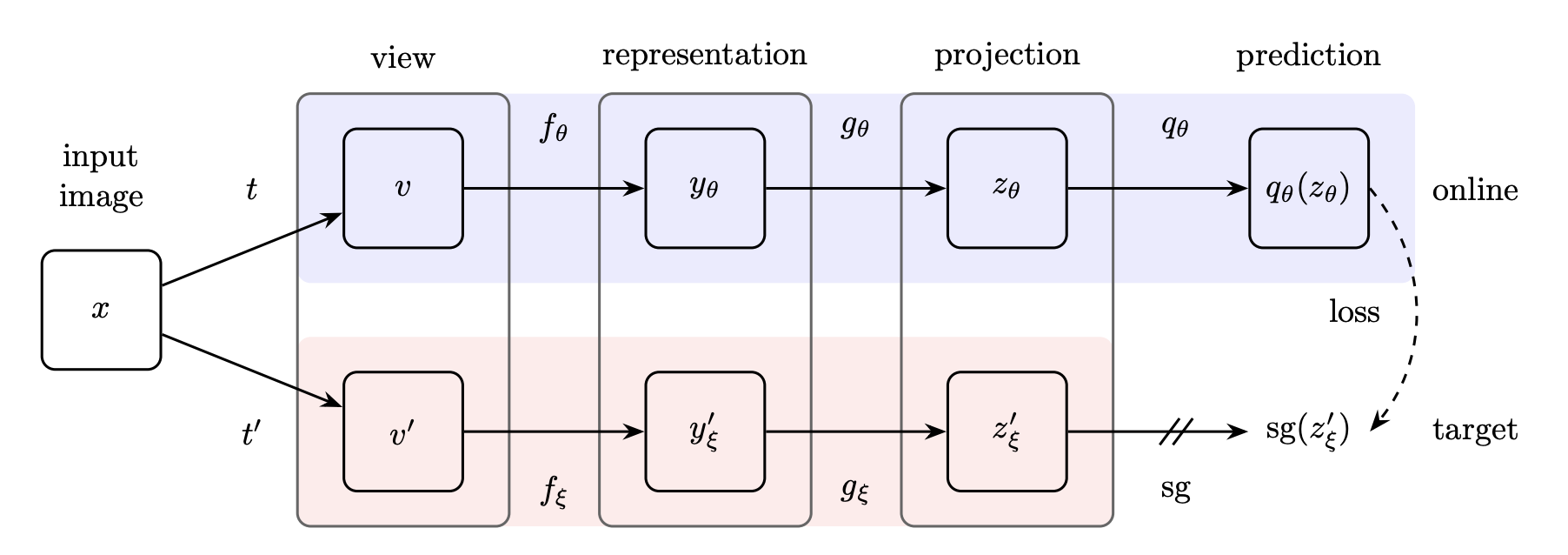
BYOL (Bootstrap Your Own Latent) is a new approach to self-supervised learning. BYOL’s goal is to learn a representation $y_\theta$ which can then be used for downstream tasks. BYOL uses two neural networks to learn: the online and target networks. The online network is defined by a set of weights $\theta$ and is comprised of three stages: an encoder $f_\theta$, a projector $g_\theta$ and a predictor $q_\theta$. The target network has the same architecture as the online network, but uses a different set of weights $\xi$. The target network provides the regression targets to train the online network, and its parameters $\xi$ are an exponential moving average of the online parameters $\theta$.
Given the architecture diagram [below], BYOL minimizes a similarity loss between $q_\theta\left(z_\theta\right)$ and $sg\left(z_{\xi}^{\prime}\right)$, where $\theta$ are the trained weights, $\xi$ are an exponential moving average of $\theta$ and $sg$ means stopgradient. At the end of training, everything but $f_\theta$ is discarded, and $y_\theta$ is used as the image representation.
Key Points
- With parallel online and target networks, they train the online network given one augmented view to predict the target network representation given another view, directly
- BYOL does not use any negative pairs (negative samples)
- Note the lack of mention of any other images in the previous bullet point: just two views of the same image
- More robust over augmentations and variations in batch size than methods which use (explicit?) negative pairs (including if those negative samples are somehow transformed, e.g. in the case of clustering-based SSL like DeepCluster)
- In particular, BYOL suffers a much smaller performance drop than SimCLR, a strong contrastive baseline, when only using random crops as image augmentations (quoted from Introduction)
- BYOL gets 74.3% accuracy on the ImageNet linear evaluation protocol with a ResNet-50 encoder6
- BYOL is good for transfer and semi-supervised downstream stuff
This paper was published after MoCo (and in fact cites it; see ref [9]) but its contribution is eliminating the negative samples that are still used by approaches like e.g. MoCo (which uses a queue of negative samples).
Background
Self-supervised methods are generative - like auto-encoding or adversarial learning - or discriminative - like contrastive learning with positive and negative samples.
They enumerate the many domain-specific pretext tasks that people tried out before contrastive methods appeared as the key paradigm for self-supervised learning:
Some self-supervised methods are not contrastive but rely on using auxiliary handcrafted prediction tasks to learn their representation. In particular, relative patch prediction [23, 40], colorizing gray-scale images [41, 42], image inpainting [43], image jigsaw puzzle [44], image super-resolution [45], and geometric transformations [46, 47] have been shown to be useful. Yet, even with suitable architectures [48], these methods are being outperformed by contrastive methods [37, 8, 12].
They mention similarity with Predictions of Bootstrapped Latents (PBL) from Bootstrap Latent-Predictive Representations for Multitask Reinforcement Learning, which trains its representation by predicting latent embeddings of future observations (see PBL Abstract). (BYOL doesn’t use a second network like PBL; it uses a momentum encoder.)
They say that using a slow-moving (e.g. momentum) encoder to encode targets comes from deep RL, citing e.g. Human-level control through deep reinforcement learning (see also references [50-53]) saying that:
Target networks stabilize the bootstrapping updates provided by the Bellman equation … [but w]hile most RL methods use fixed target networks, BYOL uses a weighted moving average of previous networks (as in [54]) in order to provide smoother changes in the target representation.
BYOL introduces an additional predictor on top of the online network, which prevents collapse.
Whereas MoCo drawn negative samples from its queue, BYOL just uses a moving-average encoder to produce prediction targets to prevent collapse.
A Note on Citations
This paper seems to do a good job of citing the work it has built on. They reference Reinforcement Learning literature (a lot from DeepMind 🤔) but also older work like Suzanna Becker and Geoffrey E. Hinton (1992) Self-organizing neural network that discovers surfaces in random-dot stereograms. Nature, which was a nice discovery when chasing up these references.
UVC: Joint-task Self-supervised Learning for Temporal Correspondence
Notes on Joint-task Self-supervised Learning for Temporal Correspondence (UVC) by Xueting Li and colleagues published in 2019.
Introduction
- correspondences between multi-view images relate 2D and 3D representations
- To learn correspondences across frames in a video, numerous methods have been developed from two perspectives: (a) learning region/object-level correspondences, via object tracking [2, 41, 43, 36, 48] or (b) learning pixel-level correspondences between multi-view images or frames, e.g., via stereo matching [34] or optical flow estimation [29, 40, 16, 31]
- not solved together
- Different annotations: bounding boxes are annotated in real videos for object tracking [52]; and pixel-wise associations are generated from synthesized data for optical flow estimation [4, 10]. Datasets with annotations for both tasks are scarcely available and supervision, here, is a further bottleneck preventing us from connecting the two tasks.
- Method: To overcome the lack of data with annotations for both tasks we exploit self-supervision via the signals of
- (a) Temporal Coherency, which states that objects or scenes move smoothly and gradually over time;
- (b) Cycle Consistency, correct correspondences should ensure that pixels or regions match bi-directionally and
- (c) Energy Preservation, which preserves the energy of feature representations during transformations
- Share affinity matrix for obj- and pixel-features
- We show that region localization and fine-grained matching can be carried out by sharing the affinity in a fully differentiable manner
- two tasks symbiotically facilitate each other: the fine-grained matching module learns better feature representations that lead to an improved affinity matrix, which in turn generates better localization that reduces the search space and ambiguities for fine-grained matching (Figure 1, right)
- Contributions:
- A joint-task self-supervision network is introduced to find accurate correspondences at different levels across video frames
- A general inter-frame transformation is proposed to support both tasks and to satisfy various video constraints: coherency, cycle, and energy consistency
- Our method outperforms state-of-the-art methods on a variety of visual correspondence tasks, e.g., video instance and part segmentation, keypoints tracking, and object tracking. Our self-supervised method even surpasses the fully-supervised affinity feature representation obtained from a ResNet-18 pre-trained on the ImageNet
Related Work
- Object-level correspondence: Our work can be viewed as exploiting the tracking-by-matching framework in a self-supervised manner
- Fine-grained correspondence:
- Dense correspondence between video frames has been widely applied for optical flow and motion estimation [31, 40, 29, 16], where the goal is to track individual pixels
- Deep optical flow mostly regresses optical flows
- direct regression of pixel offsets has limited capability for frames containing dramatic appearance changes
- Self-supervised learning: Recently, numerous approaches have been developed for correspondence learning via various self-supervised signals, including
- image transformation[17]
- color transformation [44]
- cycle-consistency
- Wang, Jabri and Efros (2019) Learning correspondence from the cycle-consistency of time. CVPR - develops patch-level tracking by modeling the similarity transformation of pixels within a fixed rectangular region
- Wang et al. (2019) Unsupervised deep tracking. CVPR - correlation filter is learned to track regions via a cycle-consistency constraint, and no pixel-level correspondence is determined
- In contrast, our method learns object-level and pixel-level correspondence jointly across video frames in a self-supervised manner.
Approach
- You can think of frames as copies one-to-another with motion augmentation
- This “copy” operator can be expressed via a linear transformation with a matrix $A$, in which $A_{i j}=1$ denotes that the pixel $j$ in the second frame is copied from pixel $i$ in the first one. An approximation of $A$ is the inter-frame affinity matrix [43, 30, 51]:
where $\kappa$ denotes some similarity function. Each entry $A_{i j}$ represents the similarity of subspace pixels $i$ and $j$ in the two frames $f_{1} \in \mathcal{R}^{C \times N_{1}}$ and $f_{2} \in \mathcal{R}^{C \times N_{2}}$, where $f \in \mathcal{R}^{C \times N}$ is a vectorized feature map with $C$ channels and $N$ pixels. In this work, our goal is to learn the feature embedding $f$ that optimally associates the contents of the two frames.
- they utilize color as a “free supervisory signal”:
- To learn the inter-frame transformation in a self-supervised manner, we can slightly modify $A_{i j}=\kappa\left(f_{1 i}, f_{2 j}\right)$ to generate the affinity via features $f$ learned only from gray-scale images
- the learned affinity is then utilized to map the color channels from one frame to another [44, 30], while using the ground-truth color as the self-supervisory signal
Problems
- One strict assumption of this formulation is that the paired frames need to have the same contents no new object or scene pixel should emerge over time
- Hence, the existing methods [44, 30] sample pairs of frames either uniformly, or randomly within a specified interval, e.g., 50 frames
- However, it is difficult to determine a “perfect” interval as video contents may change sporadically
- When transforming color from a reference frame to a target one, the objects/scene pixels in the target frame may not exist in the reference frame, thereby leading to wrong matches and an adverse effect on feature learning
- Another issue is that a large portion of the video frames are “static”, in which the sampled pair of frames are almost the same and cause the learned affinity to be an identity matrix
Solution: Incorporate a region-level localization module
- Given a pair of reference and target frames, we first randomly sample a patch in the reference frame and localize this patch in the target frame
- Interframe colour transformation is estimated between the paired patches
- Both localization and color transformation are supported by a single affinity derived from a convolutional neural network (CNN) based on the fact that the affinity matrix can simultaneously track locations and transform features
Transforming Feature and Location via Affinity
- Use top layer of e.g. ResNet-18 whose first 4 blocks take grayscale input
- Dense correspondence should have a sparse affinity matrix, but it’s hard to enforce this
- they take a more relaxed approach and apply softmax over columns
The transformation is carried out as $\hat{c_{2}}=c_{1} A$, where $A \in \mathcal{R}^{N_{1} \times N_{2}}$, and $c_{i}$ has the same number of entries as $f_{i}$ and can be features of the reference frame or any associated label, e.g., color, segmentation mask or keypoint heatmap.
Tracing pixel locations We denote $l_{j}=\left(x_{j}, y_{j}\right), l \in \mathcal{R}^{2 \times N}$ as the vectorized location map for an image/feature with $N$ pixels. Given a sparse affinity matrix, the location of an individual pixel can be traced from a reference frame to an adjacent target frame: \(l_{j}^{12}=\sum_{k=1}^{N_{1}} l_{k}^{11} A_{k j}, \quad \forall j \in\left[1, N_{2}\right]\) where $l_{j}^{m n}$ represents the coordinate in frame $m$ that transits to the $j^{t h}$ pixel in frame $n$. Note that $l^{n n}$ (e.g., $l^{11}$ in (3)) usually represents a canonical grid as shown in Figure $3 .$ 3.2 Region-level Localization In the target frame, region-level localization aims to localize a patch randomly selected from the reference frame by predicting a bounding box (denoted as “bbox”) on a region that shares matching parts with the selected patch. In other words, it is a differential region of interest (ROI) with learnable center and scale. We compute an $N_{1} \times N_{2}$ affinity $A_{p f}$ according to (2) between feature representations of the patch in the reference frame, and that of the whole target frame (see Figure $2(\mathrm{a}))$. Locating the center. To track the center position of the reference patch in the target frame, we first localize each individual pixel of the reference patch $p_{1}$ in the target frame $f_{2}$, according to (3). As we obtain the set $l^{21}$, with the same number of entries as $p_{1}$, that collects the coordinates of the most similar pixels in $f_{2}$, we can compute the average coordinate $C^{21}=\frac{1}{N_{1}} \sum_{i=1}^{N_{1}} l_{i}^{21}$ of all the points, as the estimated new position of the reference patch.
Interesting References
- Wang et al. (2019) Unsupervised deep tracking. CVPR
- Wang, Jabri and Efros (2019) Learning correspondence from the cycle-consistency of time. CVPR
SwAV: Unsupervised Learning of Visual Features by Contrasting Cluster Assignments
Notes on SwAV: Unsupervised Learning of Visual Features by Contrasting Cluster Assignments by Mathilde Caron and colleagues.
- Paper (arXiv): https://arxiv.org/pdf/2006.09882.pdf
- FAIR Blog Post: High-performance self-supervised image classification with contrastive clustering published on July 20, 2020
- Code: https://github.com/facebookresearch/swav
Related: See Caron et al.’s previous work DeepCluster and Asano et al. (2019) Self-labelling via simultaneous clustering and representation learning (reference [2]).
Summary of Contributions

Core Explanations from the FAIR Post
Headlines and Significance
We’ve developed a new technique for self-supervised training of convolutional networks commonly used for image classification and other computer vision tasks. Our method now surpasses supervised approaches on most transfer tasks, and, when compared with previous self-supervised methods, models can be trained much more quickly to achieve high performance. For instance, our technique requires only 6 hours and 15 minutes to achieve 72.1 percent top-1 accuracy with a standard ResNet-50 on ImageNet, using 64 V100 16GB GPUs. Previous self-supervised methods required at least 6x more computing power and still achieved worse performance.
Method
In this work, we propose an alternative that does not require an explicit comparison between every image pair. We first compute features of cropped sections of two images and assign each of them to a cluster of images. These assignments are done independently and may not match; for example, the black-and-white image version of the cat image could be a match with an image cluster that contains some cat images, while its color version could be a match with a cluster that contains different cat images. We constrain the two cluster assignments to match over time, so the system eventually will discover that all the images of cats represent the same information. This is done by contrasting the cluster assignments, i.e., predicting the cluster of one version of the image with the other version.
In addition, we introduce a multicrop data augmentation for self-supervised learning that allows us to greatly increase the number of image comparisons made during training without having much of an impact on the memory or compute requirements. We simply replace the two full-size images by a mix of crops with different resolutions. We find that this simple transformation works across many self-supervised methods
Related Work
Very important summary of contrastive learning for self-supervised learning via the instance discrimination task, and those tasks that essentially build on it.

DeepCluster Paper Explained on Amit Chaudhary’s amazing blog https://amitness.com/2020/04/deepcluster/

Method
In the SwAV paper, Caron et al. say:
Caron et al. [7] show that k-means assignments can be used as pseudo-labels to learn visual representations. This method scales to large uncurated dataset and can be used for pre-training of supervised network.
They mention some theory which shows DeepCluster can be cast as the optimal transport problem (by this I understand some kind of Wasserstein distance type optimisation - minimisation - criterion across image views)
Caron et al. [7, 8] and Asano et al. [2], we obtain online assignments which allows our method to scale gracefully to any dataset size.
…but they do online cluster assignments of image views, which allows scaling, since you don’t have to pass the whole dataset through the clustering algorithm once to get the cluster “codes”, used as pseudo-labels
SwAV uses a very simple pretext task:
In contrast, our multi-crop strategy consists in simply sampling multiple random crops with two different sizes: a standard size and a smaller one.
Previous work is slow because it relies on alternating between a cluster assignment and training:
Typical clustering-based methods [2, 7] are offline in the sense that they alternate between a cluster assignment step where image features of the entire dataset are clustered, and a training step where the cluster assignments, i.e., “codes” are predicted for different image views.
The crux of the SwAV method:
This solution is inspired by contrastive instance learning [58] as we do not consider the codes as a target, but only enforce consistent mapping between views of the same image. Our method can be interpreted as a way of contrasting between multiple image views by comparing their cluster assignments instead of their features.
…so in the end it is contrastive learning with multiple (image) views

This is the core method with z as features and q as code, predictable from the features if the two objects contain the same information:

This contrasts to contrastive learning since they use the swapped prediction problem (features predicting codes, given prototype codes) instead of directly comparing two sets of features:

More specifically, the loss for the Swapped Prediction task is this.
Each term represents the cross entropy loss between the code and the probability obtained by taking a softmax of the dot products of z_i and all prototypes in C.

They use an equipartition constraint when distributing samples in a batch across prototype classes to avoid collapse.
In order to compute codes online, they compute the codes using only the image features within a batch.
As the prototypes C are used across different batches, SwAV clusters multiple instances to the prototypes, that is:
We compute codes using the prototypes C such that all the examples in a batch are equally partitioned by the prototypes. This equipartition constraint ensures that the codes for different images in a batch are distinct, thus preventing the trivial solution where every image has the same code.
They enforce the equipartition constraint at the minibatch level using a transportation polytope:

What is a transportation polytope I hear you ask?

It’s just doing exactly what Caron et al. want to do, i.e. satisfy a set of margin constraints when assigning the samples across protoypes.
Have a look at these notes for more information: https://www.math.ucdavis.edu/~deloera/TALKS/20yearsafter.pdf
They would round the real polytope to get discrete prototype vectors, but this performs worse so they leave the soft targets to compute loss via cross-entropy.
When using small batch sizes, they can’t satisfy equipartitioning, so they retain features e.g. from the last 5 batches with a batch size of 256, c.f. the last 65K instances from the last 250 batches for contrastive methods that work directly on features.

multi-crop increases the self-supervised encoder’s performance, whilst keeping computational and memory cost low, since the crops are small.
Experimentally they use LARS + cosine learning rate + MLP projection head.
For more on LARS see:
- Original paper https://arxiv.org/pdf/1708.03888.pdf
- LARS at Papers with Code https://paperswithcode.com/method/lars

Some additional scribbles I made when reading the Introduction.

Up to now, this section is a stub, focussing on the introduction, background and methods. See also results section and ablation studies.
VFS: Rethinking Self-supervised Correspondence Learning A Video Frame-level Similarity Perspective
Notes on Rethinking Self-supervised Correspondence Learning A Video Frame-level Similarity by Jiarui Xu and Xiaolong Wang.
- Paper: https://arxiv.org/pdf/2103.17263.pdf
- Code: https://github.com/xvjiarui/VFS/
- Paper Website: https://jerryxu.net/VFS/
Summary
Xu and Wang propose learning correspondence by exploiting the free temporal correspondence signal directly at the frame level on the supposition that convolutional layers should learn correspondences between objects (bounding boxes in the visual object tracking; OTB) and object parts (pixel level, i.e. the DAVIS video object segmentation task; VOS).
Note: The approach(es) taken by this paper are at their core quite simple7 so the results they get are to my mind the most interesting thing about this paper, especially the quirky but intuitive result they get which shows that colour augmentations affect pixel-level label propagation performance negatively but improve object-level tracking.
Main Results
They summarise their main results:
- Large frame gaps and multiple frame pairs improves correspondence
- Fine-grained by ~3% (DAVIS)
- Object-level by > 10% (OTB)
- Training with multiple frame pairs simultaneously improves performance even more.
- I guess they mean constructing an affinity matrix with multiple positive pairs (see Pipeline)
- Colour augmentation is harmful for fine-grained correspondence (~3% DAVIS), but beneficial for object-level correspondence (~10% OTB; ‘future learns better object invariance’)
- Training without negative pairs improves both object-level and fine-grained performance - very surprising result!
- Deeper models exhibit better performance - SSL pretext task training for correspondence usually renders deeper nets redundant, meaning performance doesn’t improve going deeper e.g. ResNet-50 vs ResNet-18. But training with VFS’ pretext task using video frames does show improved (downstream) performance for deeper nets.
Approach
Their method is actually very simple, since it just straightforwardly applies contrastive methods from visual representation learning to video frames, leveraging the inherent augmentation of motion across time to learn using a similarity loss. In particular, they ‘unify’ methods with negative pairs, like SimCLR and MoCo, and ones without negative pairs, like BYOL and especially SimSiam. In doing this, they question (or even undermine) the utility of more elaborate object- or patch-tracking pretext task set-ups for learning correspondences, asking:
Do we really need to design self-supervised object (or patch) tracking task explicitly to learn correspondence? Can image-level similarity learning alone learn the correspondence?
They apply standard image augmentations on top of the selection of frames across time. This is especially interesting since they observe using colour augmentation is harmful for fine-grained correspondence (pixel-level; DAVIS VOS) but beneficial for object-level correspondence (OTB).
So basically, given two frames (or more pairs) sampled according to either strategy, possibly with additional augmentation they forward them to the predictor encoder, $\mathcal{P}$, and the target encoder, $\mathcal{T}$, do $l_2$ normalisation of the output representation8 and either…
use InfoNCE loss (from the CPC paper), like so
\[\mathcal{L}_{p_{i}, z_{j}, \mathcal{U}}=-\log \frac{\exp \left(p_{i} \cdot z_{j} / \tau\right)}{\exp \left(p_{i} \cdot z_{j} / \tau\right)+\sum_{k=1}^{K} \exp \left(p_{i} \cdot u_{k} / \tau\right)}\]or they don’t use negative pairs (SimSiam, BYOL) and minimise the loss
\[\mathcal{L}_{p_{i}, z_{j}}=\left\|p_{i}-z_{j}\right\|_{2}^{2}=2-2 \cdot p_{i} \cdot z_{j}\]Implementation
It’s nice because they unify the with negative pairs and without negative pairs approaches but using very consistent implementation, which they take directly from Xinlei Chen and Kaiming He (along with those guys’ colleagues) so they use
- With Negative Pairs: Improved baselines with momentum contrastive learning - this is the extension paper to MoCo, let’s say MoCo v2
- Without Negative Pairs: Exploring simple siamese representation learning - SimSiam
(Pre-)Training (emphasis mine):
We adopt the Kinetics [41] dataset for self-supervised training. It consists of ∼240k training videos. The batch size is 256. The learning rate is initialized to 0.05, and decays in the cosine schedule [12, 49, 13]. We use SGD optimizer with momentum 0.9 and weight decay 0.0001. We found that training for 100 epochs is sufficient for ResNet-18 models, and ResNet-50 models need 500 epochs to converge (roughly the same number of iterations as 100 epochs training [14] on ImageNet).
Pipeline

The affinity matrix is the pairwise feature similarity between predictor features and target features.
The dash rectangle areas indicate the with negative pairs case. [Negative pairs are one of the two research streams they pursue to train their model. Remember that you can use stop-grad like SimSiam or a momentum encoder like BYOL.]
The features of negative samples are stored in the negative bank [like MoCo, which uses a “queue” of negative samples in conjunction with a momentum encoder] and concatenate with target features.
The encoder is trained to maximize the affinity of positive pairs and minimize the affinity of negative ones.
Video Frame Sampling
Continuous sampling: They either sample over constant intervals, $\delta$, - from a video of length $L$ to get frames $I_i \in [1, L]$ or…
Distant sampling: Split the length-$L$ video into $n$ disjoint segments and take a random frame from each segment randomly, according to $I_{i}=\frac{L}{n}(i-1)+\operatorname{unif}\left(0, \frac{L}{n}\right)$

Sidenote: They comment that continuous (consistent) sampling is more common when using 3D Convolution as used in Learning spatiotemporal features with 3d convolutional networks or Quo Vadis, Action Recognition? A New Model and the Kinetics Dataset.
Augmentations
- Spatial: Random cropping and flipping
- Colour augmentation: grayscale and colour jitter - Affects OTB vs VOS downstream performance, see Main Results
Results
First a few details:
- Fine-grained correspondence:
- fine-grained similarity is measured on the $\text{res}_4$ feature map, with its stride reduced to 1 during inference
- Recurrent inference strategy used: First ground-truth frame and latest 20 predicted frames are propagated to the current frame
- DAVIS for VOS, pose-tracking done in JHMDB and human-part tracking in VIP
- Object-level correspondence:
- evaluate object-level correspondence with visual object tracking in the OTB-100 [78] dataset
- they use SiamFC tracking with the representation from their trained res$_5$ block
- Given the pretrained ResNet, the strides in res$_4$ and res$_5$ are removed and dilations of 2 and 4 are added to these block respectively - makes the res$_5$ block output compatible with SiamFC but does not affect the pretrained weights
- Most of their analysis is on a frozen ResNet then comparisons to SotA is with fine-tuning (end of paper)
Results: Downstream Performance on DAVIS and OTB

- Colour augmentation helps object-level and harms pixel-level correspondence
- Spatial augmentations help both
- Temporal sampling further apart (with a constant step) is better, and sampling according to the distant sampling (uniform in a segment) approach is best (with 2 disjoint segments, i.e. 2 frames)
- Using more frames from a single video is better
- Using negative pairs worsens performance
What is the reason causing this performance drop when training with negatives?
Our hypothesis is that training with negative pairs may sacrifice the performance on modeling intra-instance invariance for learning better features for cross instance discrimination.
To prove this hypothesis, we perform linear classification on top of the frozen features on the ImageNet-1k dataset [18] and report the results on the right column of Table 5.
We observe that the model trained with negatives indeed leads to better semantic classification with around 2% improvement, which supports our hypothesis.
- Different blocks of the res$_4$ and res$_5$ layers specialise in a sense
- res$_4$ is better at fine-grained correspondence tasks
- res$_5$ focuses on object-level
They evaluate J&F mean scores on DAVIS at different epochs using the features of different blocks from the res$_4$ and res$_5$ layers as a nice ablation study

Comparison to SotA
VFS outperforms all SotA benchmarks on object-level tasks with ResNet-18 or ResNet-50 backbones.

For the fine-grained correspondence, they surpass all SotA benchmarks except Contrastive Random Walk (CRW; or “Videowalk”) for ResNet-18, and for ResNet-50 they are always best, although they don’t compare against CRW because they couldn’t get the architecture to work for the deeper backbone.
Additional Notes
Some additional small points.
SyncBN
They use Synchronised Batch Normalisation, which is batch norm used for multi-GPU training wherein the batch norm statistics (mean and standard deviation) are calculated across the whole minibatch, i.e. across all the GPUs used for training.
This is different from what would happen otherwise, where the statistics would only by computed within each GPU. (Remember that when you set the batch size in PyTorch when using multiple GPUs for training, you in practice send a minibatch of size $\text{batch size} / N_\text{GPUs}$ to each GPU.)
You can use SyncBatchNorm with torch.nn.SyncBatchNorm which applies batch norm but ensures [t]he mean and standard-deviation are calculated per-dimension over all mini-batches of the same process groups.
See also the PyTorch SyncBatchNorm source code and Zhang et al. Context Encoding for Semantic Segmentation, which made use of it for the first time.
Authors’ Conclusions
1. Tracking-based pretext tasks are not necessary for self-supervised correspondence learning
Is designing a tracking-based pretext task a necessity for self-supervised correspondence learning? It might not be necessary. While tracking-based pretext tasks still have potentials, it is limited by small backbone models and is now surpassed by our simple frame-level similarity learning. To make the tracking-based pretext tasks useful, we need to first make its learning scalable and generalizable in model size and network architectures.
2. Colour augmentation improves object tracking and worsens pixel-level tracking
color augmentation is beneficial for correspondence in object-level but jeopardizes the fine- grained correspondence. While color augmentation brings object appearance invariance, it also confuses the lower- layer convolution features
3. Sample multiple frames and sample with a large gap
The large temporal gap provides more aggressive temporal transform, which boosts correspondence significantly. Comparing multiple pairs of frame further improves the results
4. Negative pairs decrease performance, let alone being not necessary for contrastive learning when learning via self-supervised correspondence
We observe inferior performance when training with negative samples, specifically for object-level correspondence. We also shed light on the reason why without negative pairs is more helpful, which has not been studied before
Implementation
Watch out for the strange structure of the VFS repository, that uses MMCV (a tool I haven’t personally used at the time of writing, but which looks useful for modularising tests and model builds) to do the model builds.
The models reside in VFS/mmaction/models but are built with (what are in the end calls to) the build function in builder.py in that directory.
-
Raia Hadsell, Sumit Chopra, and Yann LeCun. Dimensionality reduction by learning an invariant mapping. In CVPR, 2006 ↩
-
“Logits” in the deep learning sense actually doesn’t correspond to logits in the actual, statistics sense where it means the log of the odds. Instead logits in the context of neural networks means the raw, unnormalised network outputs (e.g. before the softmax layer). ↩
-
0.3% accuracy is reported when removing the momentum encoder; see Table 5 of the BYOL paper. In BYOL’s arXiv v3 update, it reports 66.9% accuracy with 300-epoch pre-training when removing the momentum encoder and increasing the predictor’s learning rate by 10×. Our work was done concurrently with this arXiv update. Our work studies this topic from different perspectives, with better results achieved. ↩
-
A stop-gradient is required for a momentum-encoder because the momentum-encoder’s weights are updated as an exponential moving average of the current and previous iterations’ encoder weights from the other branch of the networks, which gradients backpropagate through. So obviously this update is done independently of any gradients that flow back through the momentum-encoder branch of the network / the set-up. That said, as the authors (of SimSIam) say _even though MoCo [17] and BYOL [15] do not directly share the weights between the two branches, … the momentum encoder should converge to the same status as the trainable encoder [so] these models [can be viewed] as Siamese networks with “indirect” weight-sharing. 🤭 ↩
-
Remember, we’re talking about an output representation from a vision encoder, so vector elements are output channels. ↩
-
Using a bigger ResNet encoder, they get the benchmark accuracy up to 79.6% ↩
-
…and borrow heavily from MoCo and SimSiam (along with related papers) for the method and implementation, but they apply this using video… ↩
-
Remember that it is very important to norm the output representations of networks when using contrastive losses, since otherwise you are allowing the different magnitudes of the representation vectors (and their elements) to count in facilitating discrimination between positive and negative pairs. (In the case where no negative pairs are used, I suppose there’s some implicit mechanism that renders this a problem for analogous reasons.) ↩