CPC: Representation Learning with Contrastive Predictive Coding
Notes on Representation Learning with Contrastive Predictive Coding (CPC) by Aaron van den Oord, Yazhe Li and Oriol Vinyals.
- Paper: https://arxiv.org/pdf/1807.03748.pdf
- Code (PyTorch): https://github.com/jefflai108/Contrastive-Predictive-Coding-PyTorch
- Code contains
CDCK2base model but see also Implementation for details on variations (changing encoder or decoder) of the base model - Papers with Code: https://paperswithcode.com/method/contrastive-predictive-coding
- A glossary is at the end in case you need it for the post
Summary
CPC is a new method that combines predicting future observations (predictive coding) with a probabilistic contrastive loss (Equation 4). This allows us to extract slow features, which maximize the mutual information of observations over long time horizons. Contrastive losses and predictive coding have individually been used in different ways before
Contrastive Predictive Coding (“CPC”) is a universal unsupervised approach for high-dimensional data that works by predicting the future (i.e. discrete future observations) in a latent space using autoregressive models. It uses a probabilistic contrastive loss based on Noise-Contrastive Estimation (NCE), called InfoNCE that induces the latent space to capture maximally useful information for prediction (forecasting). InfoNCE (like NCE) leverages negative sampling. CPC is a modality-agnosic framework that you can apply to speech, images, text, RL for 3D environments, and they do this in the paper. They target challenges around data efficiency, representation robustness and generalization across downstream tasks.
Method
- compress high-dimensional data into compact latent embedding in which conditional predictions are easier to model
- Use powerful autoregressive models (in latent space) to predict many (time) steps into the future
- Use Noise-Contrastive Estimation (NCE) for loss function (like word embeddings) for end-to-end training
- Apply resulting CPC model to images, speech, NLP, RL to show it works in multiple domains / modalities

Motivations / Intuitions
- Learn representations that encode shared information between parts of the signal
- Slow features more useful at long timespan (far out) predictions e.g. intonation, objects, story line
- Information in input $x$ e.g. an image may be e.g. thousands of bits, whereas class labels could be e.g. 10 bits (1,024 classes) so modelling $o(x \vert c)$ may be suboptimal for extracting shared information
- Instead authors encode target $x$ (future) and context $c$ (present) into compact distributed vector representations to maximally preserve mutual information of the original signals $x$ and $c$ as:
By maximising the mutual information (MI) between encoded representations (bounded by the MI between input signals) they extract the underlying latent variables that the inputs have in common.
Contrastive Predictive Coding Algorithm / Method
- Encoder net, $g_\text{enc}$, maps input sequence $x_t$ to sequence of latent representations, $z_t = g_\text{enc}(x_t)$ also possibly with lower temporal resolution
- Autoregressive model, $g_\text{ar}$ summarises $z_{\leq t}$ (latent reps sequence) producing single vector representation, $c_t = g_\text{ar}(z_{\leq t})$ (also in latent space)
They don’t predict with a generative model, $p_k(x_{t+k} \vert c_t)$.
They model a density ratio preserving the mutual information between the AR-generated latent representation, $c_t$ and the future observations, $x_{t+k}$
\[f_{k}\left(x_{t+k}, c_{t}\right) \propto \frac{p\left(x_{t+k} \mid c_{t}\right)}{p\left(x_{t+k}\right)}\]NB the density ratio, $f$, can be unnormalized, i.e. does not have to integrate to 1.
Although any positive real score can be used, they use a log-bilinear model with the addition of a linear transformation for each prediction step, $k$, via $W_k$:
\[f_{k}\left(x_{t+k}, c_{l}\right)=\exp \left(z_{l+k}^{T} W_{k} c_{l}\right)\]Using the density ratio and using the encoded representations frees the model from learning the high-dimensional distribution of $x_{t_k}$.
They can’t evaluate $p(x)$ or $p(x \vert c)$ directly, but instead sample from those distributions and so can use Noise-Contrastive Estimation or Importance Sampling to train the model by comparing the target value (distribution) with (the distribution of) randomly sampled negative values.
- you can choose $z_t$, the present time representation, or $c_t$ the summary representing the past up to now to do prediction
- the summary might work better for e.g. speech recognition which needs a bigger receptive field
- the instantaneous representation might work better elsewhere (…but where?)
- the choice of summariser (autoregressive or otherwise) and encoder are up to you (you can swap them out, e.g. use attention or a TCN for the AR summariser)
- they chose a ResNet encoder and a GRU (AR-)summariser
InfoNCE Loss and Mutual Information Estimation
They base their InfoNCE loss for jointly training the encoder and (AR-)summariser on Noise-Contrastive Estimation (NCE)
Given a set $X=\left\{x_{1}, \dots, x_{N}\right\}$ of $N$ random samples containing one positive sample from $p\left(x_{t+k} \mid c_{t}\right)$ and $N-1$ negative samples from the ‘proposal’ distribution $p\left(x_{t+k}\right)$, they optimize the loss:
\[\mathcal{L}_{\mathrm{N}}=-\underset{X}{\mathbb{E}}\left[\log \frac{f_{k}\left(x_{t+k}, c_{t}\right)}{\sum_{x_{j} \in X} f_{k}\left(x_{j}, c_{t}\right)}\right]\]Optimizing this loss $f_{k}\left(x_{t+k}, c_{t}\right)$ estimates the density ratio that preserves the mutual information between the context vector $c_t$ and the future observations, $\frac{p\left(x_{t+k} \mid c_{t}\right)}{p\left(x_{t+k}\right)}$.
Here’s why.
Proof that InfoNCE Estimates the Mutual Information Density Ratio
- The InfoNCE loss is the categorical cross-entropy of classifying the positive sample correctly, with $\frac{f_{k}}{\sum_{X} f_{k}}$ being the prediction of the model.
- The optimal probability for this loss is $p\left(d=i \mid X, c_{t}\right)$ where $[d=i]$ is the indicator that sample $x_{i}$ is the ‘positive’ sample.
- The probability that sample $x_{i}$ was drawn from the conditional distribution $p\left(x_{t+k} \mid c_{t}\right)$ rather than the proposal distribution $p\left(x_{t+k}\right)$ can be derived as follows (taken directly from the paper):
As we can see, the optimal value for $f\left(x_{t+k}, c_{t}\right)$ in [the expression for the InfoNCE loss] is proportional to $\frac{p\left(x_{t+k} \mid c_{t}\right)}{p\left(x_{t+k}\right)}$ and this is independent of the the choice of the number of negative samples $N-1$.
Though not required for training, we can evaluate the mutual information between the variables $c_{t}$ and $x_{t+k}$ as follows:
\[I\left(x_{t+k}, c_{t}\right) \geq \log (N)-\mathcal{L}_{\mathrm{N}}\]which becomes tighter as $\mathrm{N}$ becomes larger. Also observe that minimizing the InfoNCE loss $\mathcal{L}_{\mathrm{N}}$ maximizes a lower bound on mutual information.
For more details see the paper’s Appendix.
Related Work
- Contrastive losses had been used e.g. triplet loss with max-margin to repel and attract negatives and positives respectively
- Time Contrastive Networks using contrastive losses to do self-supervised learning from video1
- Triplet loss in computer vision on positive (tracked) patches and negative (random) patches
- Prediction tasks:
- Word2Vec
- Skip-thought vectors and Byte mLSTM: go beyond word-level (granularity) using RNN over sequences
Results
Audio
- 100-hour subset of the publicly available LibriSpeech dataset with force-aligned phone sequences (has speech from 251 speakers)
- $g_\text{enc}$ was strided ConvNet runs directly on 16KHz audio waveform
- Downsampling is 160 $\rightarrow$ feature vector for every 10ms of speech (matches phone sequence label rate)
- GRU RNN for AR summariser (256D hidden state)
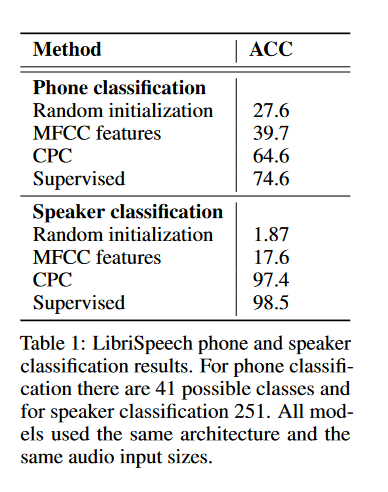
- Evaluate phone prediction performance with linear classifier over features using $c_t$ from GRU (256-dimensional) with a “multi-class linear logistic regression classifier” (just a softmax??) on top
Results:
When they used a single hidden layer (projection head) instead of keeping the classifier linear, the accuracy increases from 64.6 to 72.5, i.e. closer to the accuracy of the fully supervised model.
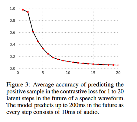
Prediction (they predict the latent representation $k$ steps away) becomes harder as you get further away (max time into the future is 200ms since a step is 10ms of raw audio)
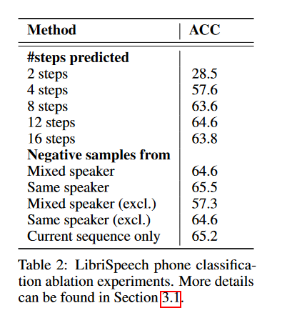
Audio Ablation
Seems to be best to predict 12 steps out and use negative samples from the same speaker, or even only the current sequence (by default the same speaker)
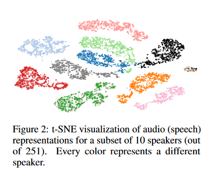
The model also learns to discriminate speaker voices, as shown by the t-SNE (a non-linear dimensionality reduction - and therefore useful visualisation - technique).
Vision
- ImageNet + ResNet v2 101 as $g_\text{enc}$ (not pretrained)
Training
- from a 256x256 image extract a 7x7 grid of 64x64 crops with 32 pixels overlap (like in Space-Time Correspondence as a Contrastive Random Walk)
- Simple data augmentation proved helpful on both the 256x256 images and the 64x64 crops:
- The 256x256 images are
- randomly cropped from a 300x300 image
- horizontally flipped with a probability of 50%
- converted to greyscale
- For each of the 64x64 crops they randomly take a 60x60 subcrop and pad them back to a 64x64 image
- The 256x256 images are
- Each crop is then encoded by the ResNet-v2-101 encoder
- The outputs from the third residual block are spatially mean-pooled to get a single 1024-d vector per 64x64 patch
- This results in a 7x7x1024 tensor
- They use a PixelCNN-style autoregressive model as per Conditional Image Generation with PixelCNN Decoders2 to make predictions about the latent activations in the following rows top-to-bottom - See picture below! “Vision Prediction Task”
- We predict up to five rows from the 7x7 grid, and we apply the contrastive loss for each patch in the row3
Vision Prediction Task
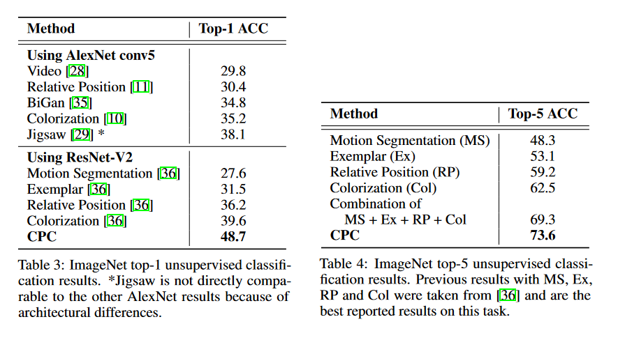
They get state-of-the-art - for unsupervised - results.
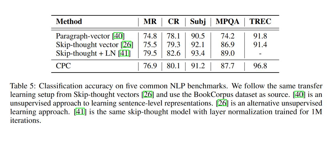
Natural Language
They follow Skip-thought vectors4.
Training
- train a logistic regression classifier and evaluate with 10-fold cross-validation for MR, CR, Subj, MPQA
- Encoder $g_\text{enc}$: 1D Conv + ReLU + Mean-Pooling $\rightarrow$ 2400-dimensional embedding $z$
- GRU (2400D hidden state)
- Predicts up to 3 future sentence embeddings with contrastive loss to give $c$
Results
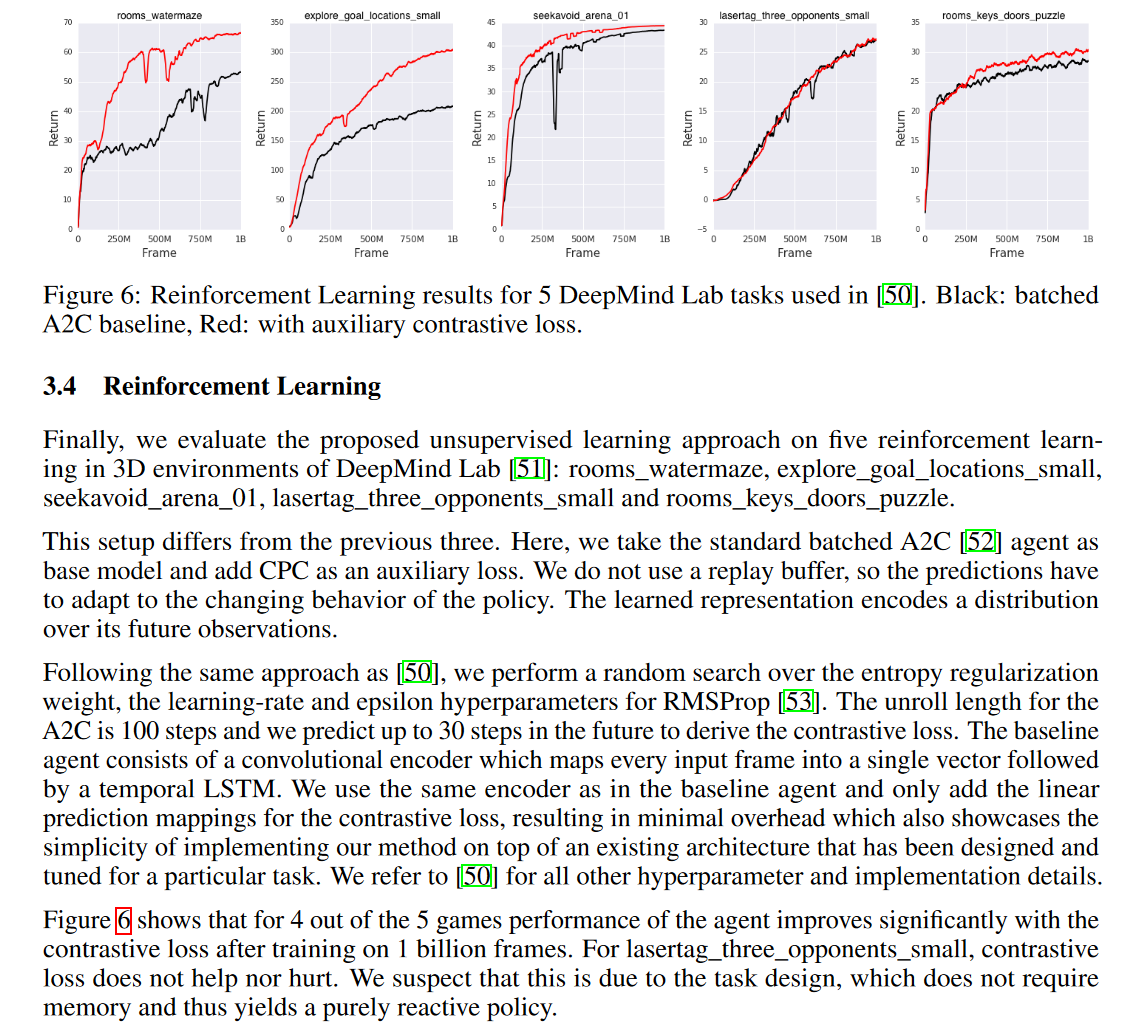
Reinforcement Learning
I’m not so familiar with RL but I wanted to include this section in case I need to refer back to it.
Important Refs
- [04] Show and tell: A neural image caption generator
- [12] Michael Gutmann and Aapo Hyvärinen (2010) Noise-contrastive estimation: A new estimation principle for unnormalized statistical models Noise-Contrastive Estimation - Seminal NCE paper that I find quite hard to understand
- [14] Andriy Mnih and Yee Whye Teh (2012) A fast and simple algorithm for training neural probabilistic language models (published at ICML) - This paper explains Noise-Contrastive Estimation much better than the original and derives NCE then applies it in the context of Language Modelling (where they test it for sentence completion and other tasks)
- Noise-Contrastive Estimation explained quite well - Lei Mao’s blog post which explains NCE very clearly and borrows heavily from Mnih and Teh (2012; above)
- [15] Rafal Jozefowicz, Oriol Vinyals, Mike Schuster, Noam Shazeer, and Yonghui Wu (2016) Exploring the limits of language modeling
Additional Stuff
Log-bilinear Models
Log-bilinear models were popular for language modelling.
They are a simple model which takes as input the history of words as latent representations, combines these representations linearly to form a “context vector” and then produces a probability distribution - and therefore prediction - for the next element (e.g. word) based on computing the similarity between the context representation and all elements (words) in the vocabulary.
The following is the explanation of log-bilinear models given by Geoff Hinton in his lecture (page 9; hierarchical log-bilinear models are explained on page 13):
The log-bilinear (LBL) model is perhaps the simplest neural language model.
Given the context $w_{1: n-1}$, the LBL model first predicts the representation for the next word $w_{n}$ by linearly combining the representations of the context words:
\[\hat{r}=\sum_{i=1}^{n-1} C_{i} r_{w_{i}}\]NB $r_{w}$ is the real-valued vector representing word $w$
Then the distribution for the next word is computed based on the similarity between the predicted representation and the representations of all words in the vocabulary:
\[P\left(w_{n}=w \mid w_{1: n-1}\right)=\frac{\exp \left(\hat{r}^{T} r_{w}\right)}{\sum_{j} \exp \left(\hat{r}^{T} r_{j}\right)}\]Glossary
- AR: Autoregressive
- MI: Mutual information
- NCE: Noise-Contrastive Estimation
- TCN: Temporal convolutional network
Authors’ Acknowledgements
We would like to thank Andriy Mnih, Andrew Zisserman, Alex Graves and Carl Doersch for their helpful comments on the paper and Lasse Espeholt for making the A2C baseline available.
Summary from Papers with Code
Contrastive Predictive Coding (CPC) learns self-supervised representations by predicting the future in latent space by using powerful autoregressive models. The model uses a probabilistic contrastive loss which induces the latent space to capture information that is maximally useful to predict future samples.
First, a non-linear encoder $g_{e n c}$ maps the input sequence of observations $x_{t}$ to a sequence of latent representations $z_{t}=g_{e n c}\left(x_{t}\right)$, potentially with a lower temporal resolution. Next, an autoregressive model $g_{a r}$ summarizes all $z \leq t$ in the latent space and produces a context latent representation $c_{t}=g_{a r}(z \leq t)$ A density ratio is modelled which preserves the mutual information between $x_{t+k}$ and $c_{t}$ as follows:
\(f_{k}\left(x_{t+k}, c_{t}\right) \propto \frac{p\left(x_{t+k} \mid c_{t}\right)}{p\left(x_{t+k}\right)}\) where $\propto$ stands for ‘proportional to’ (i.e. up to a multiplicative constant). Note that the density ratio $f$ can be unnormalized (does not have to integrate to 1). The authors use a simple log-bilinear model: \(f_{k}\left(x_{t+k}, c_{t}\right)=\exp \left(z_{t+k}^{T} W_{k} c_{t}\right)\)
Any type of autoencoder and autoregressive can be used. An example the authors opt for is strided convolutional layers with residual blocks and GRUs.
The autoencoder and autoregressive models are trained to minimize an InfoNCE loss (see components).
Implementation
Implementation in PyTorch from Cheng-I Jeff Lai contains a few different model classes in Contrastive-Predictive-Coding-PyTorch/src/model/model.py.
PyTorch implementation of CDCK2, CDCK5, CDCK6, speaker classifier models:
- CDCK2: base model from the paper ‘Representation Learning with Contrastive Predictive Coding’
- CDCK5: CDCK2 with a different decoder
- CDCK6: CDCK2 with a shared encoder and double decoders
- SpkClassifier: a simple NN for speaker classification
Notes
-
From Time-Contrastive Networks: Self-Supervised Learning from Video by Pierre Sermanet and colleagues published in 2017 (revised most recently in 2018). The authors train [their] representations using a metric learning loss, where multiple simultaneous viewpoints of the same observation are attracted in the embedding space, while being repelled from temporal neighbors which are often visually similar but functionally different. In other words, the model simultaneously learns to recognize what is common between different-looking images, and what is different between similar-looking images. This signal causes our model to discover attributes that do not change across viewpoint, but do change across time, while ignoring nuisance variables such as occlusions, motion blur, lighting and background. ↩
-
a convolutional row-GRU PixelRNN gave similar results ↩
-
[They] used Adam optimizer with a learning rate of 2e-4 and trained on 32 GPUs each with a batch size of 16 ↩
-
Ryan Kiros, Yukun Zhu, Ruslan R Salakhutdinov, Richard Zemel, Raquel Urtasun, Antonio Torralba, and Sanja Fidler. Skip-thought vectors. In Advances in neural information processing systems, pages 3294–3302, 2015 ↩